set.seed(696)

rho <- 0.6

gibbs_step <- function(x){
  x[1] <- rnorm(1, rho * x[2], sqrt( 1-rho^2 ) )
  x[2] <- rnorm(1, rho * x[1], sqrt( 1-rho^2 ) )
  return(x)
}

num_samples <- 10000
x_all_samples <- matrix(NA, ncol=2, nrow=num_samples)
colnames(x_all_samples) <- c("X1", "X2")

x <- c(0,0) # initial value

# run the Gibbs sampler
for(i in 1:num_samples){
  x <- gibbs_step(x)
  x_all_samples[i,] <- x
}Bayesian Regression with Gaussian Processes
Spatial Statistics - BIOSTAT 696/896
University of Michigan
From response model to regression with latent GP
- We have considered (ML) inference of the following model
Y(\cdot) \sim GP(0, C_{\theta}(\cdot, \cdot))
- Optimizing becomes more difficult as we increase the dimension of \theta
- We may want to model a non-zero mean based on covariate matrix X
- We may want to make the model more complex or flexible
Bayesian linear regression with latent GP
- Linear regression model with spatial random effects
- Spatial random effects = unobserved error term with spatial correlation
- Equivalent to having correlated measurement error
- Separate purely spatial error from purely noise error terms
At location s, we model
Y(s) = X(s)^\top\beta + w(s) + \varepsilon(s)
- X(s) is a p\times 1 vector of covariates at location s
- \beta is a constant vector of regression coefficients
- w(s) is the realization at s of a GP
- \varepsilon(s) is independent noise
Model DAG
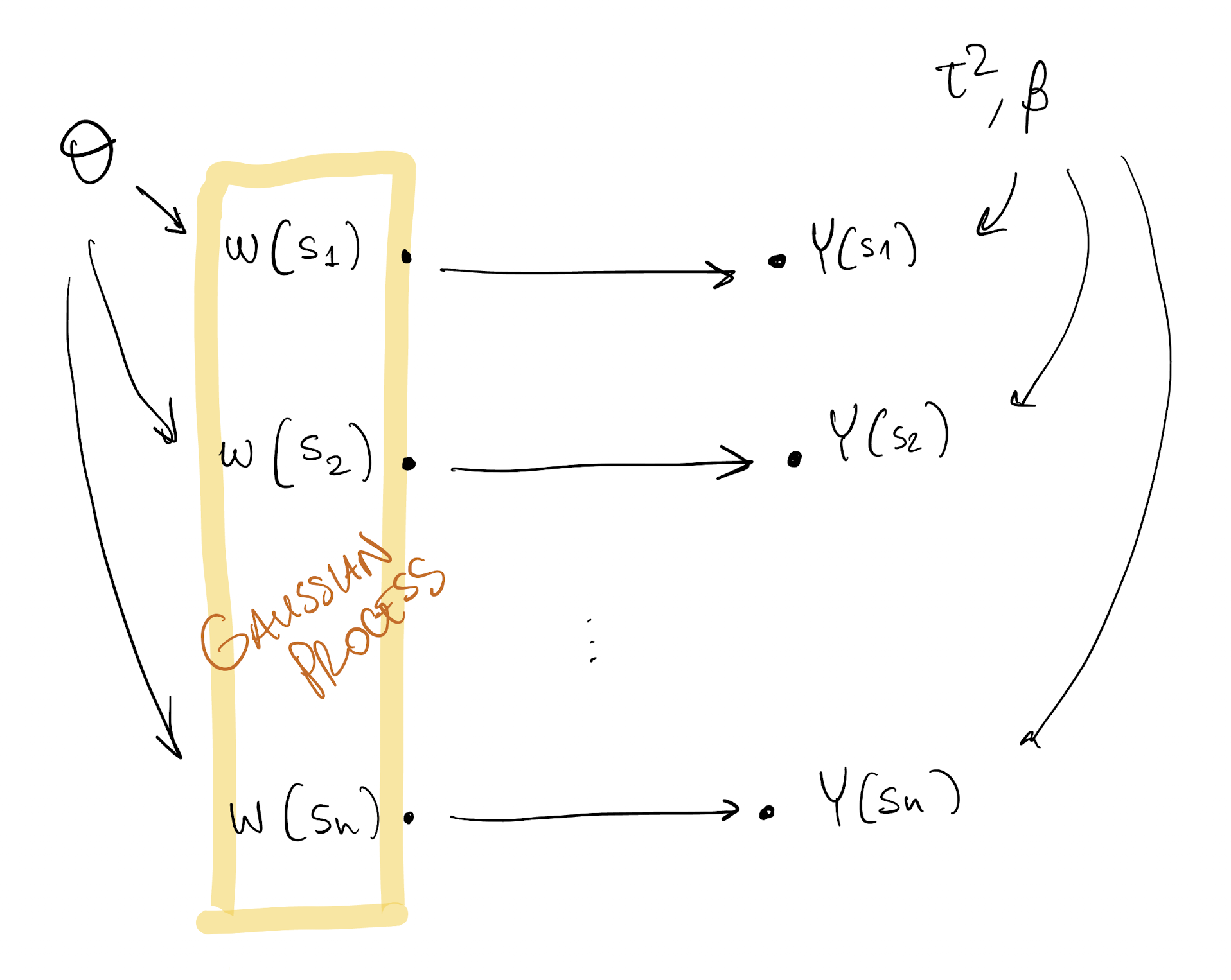
Model DAG
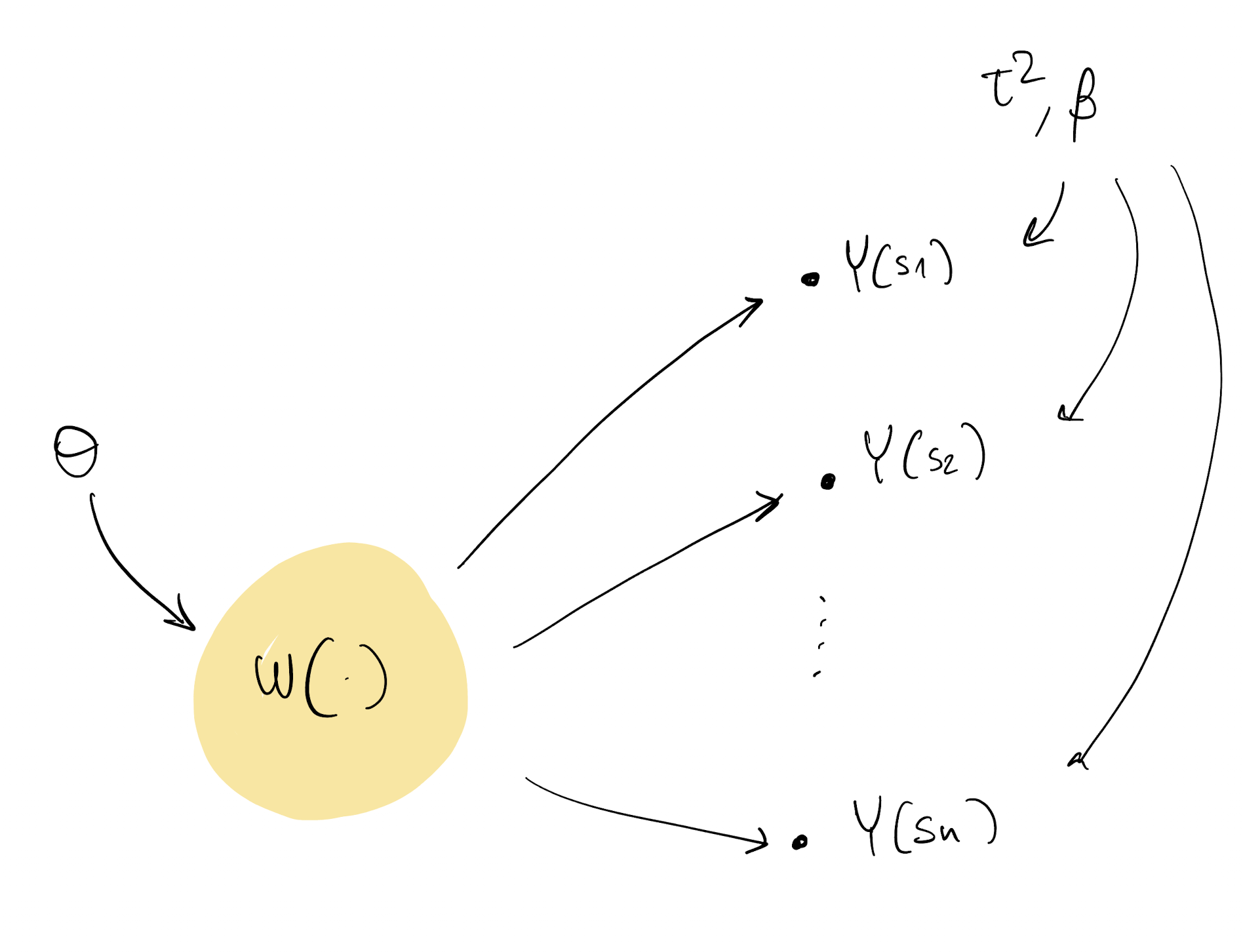
Bayesian linear regression with latent GP
At location s, we model
Y(s) = X(s)^\top\beta + w(s) + \varepsilon(s)
X(s) is a p\times 1 vector of covariates at location s
\beta is a constant vector of regression coefficients
w(s) is the realization at s of a GP: we assume w(\cdot) \sim GP(0, \tau^2 C_{\theta}(\cdot, \cdot) ) where we have included \tau^2 for conjugacy
Example: C_{\theta}(s, s') = s^2 \exp\{ -\phi \| s-s' \| \} and the process variance can be computed as
Var(w) = Cov(w(s), w(s)) = \tau^2 s^2
Notice: if we denote Var(w) = \sigma^2 then \sigma^2 = \tau^2 s^2 and we interpret s^2 as the signal-to-noise ratio
\text{SNR:} \qquad s^2 = \frac{\sigma^2}{\tau^2}
- \varepsilon(s) is iid noise \varepsilon(s) \sim N(0, \tau^2)
- We do not need a nugget term in C_{\theta}(\cdot, \cdot) as we are including iid noise in our model
Bayesian linear regression with latent GP
Take \cal T as the set of observed locations, then the model can be written as
Y = X\beta + w + \varepsilon where Y, X, w and \varepsilon are vectors and matrices with appropriate dimensions.
- We call this a latent GP model because we are explicitly introducing latent (unobserved) variables (i.e., each element of w)
- Let’s assign conjugate priors to most unknown parameters:
- GP assumption implies w \sim N(0, \tau^2 C_{\theta})
- The prior on \theta is not conjugate: write generically \theta \sim p(\theta) (we will specify later)
Bayesian linear regression with latent GP
Priors:
\begin{align*} \theta &\sim p(\theta) \\ \tau^2 &\sim Inv.G(a, b) \\ \beta | \tau^2 &\sim N(0, \tau^2 V_{\beta}) \\ \text{at}\ \cal T \ \text{:}\qquad w &\sim N(0, \tau^2 C_{\theta}) \qquad \text{because} \qquad w(\cdot) &\sim GP(0, \tau^2 C_{\theta}(\cdot)) \end{align*}Model/Likelihood:
Y | \beta, w, \tau^2 \sim N(X \beta + w, \tau^2 I_n)
Posterior we want to find:
p(\beta, \theta, \tau^2 | Y) = \text{???}
Bayesian linear regression with latent GP
Posterior we want to find:
p(\beta, \theta, \tau^2 | Y) = \text{???}
- w are “nuisance” parameters. They are “in the way” when estimating \theta a posteriori
- p(w|Y) is the posterior of the GP, which we will need to make predictions at new locations
p(w | Y) = \int p(w, \beta, \theta, \tau^2 | Y)d\beta, d\theta, d\tau^2 = \int p(w | Y,\beta, \theta, \tau^2)p(\beta, \theta, \tau^2 | Y)d\beta, d\theta, d\tau^2
- Therefore, once again we first need p(\beta, \theta, \tau^2 | Y)
- Notice: p(w | Y, \beta, \theta, \tau^2) is the conditional posterior for fixed values of \beta, \theta, \tau^2
- We have a roadmap, now we will work towards finding p(\beta, \theta, \tau^2 | Y)
Finding p(\beta, \theta, \tau^2 | Y)
- We marginalize over w (aka integrate out w) and get the marginal likelihood
p(Y | \beta, \theta, \tau^2) =\int p(Y, w| \beta, \theta, \tau^2) dw = \int p(Y | \beta, w, \theta, \tau^2) p(w | \theta) dw
With Gaussian things, this is easy! If U \sim N(m_U, S_U) independent of V \sim N(m_V, S_V) and Z = U + V + \varepsilon where \varepsilon \sim N(0, a I_n) then Z|U,V \sim N(U + V, aI_n), Z|U \sim N(U + m_V, S_V + aI_n), Z \sim N(m_U + m_V, S_U + S_V + aI_n).
In our case, the Gaussisan things are \beta, w, and Y, therefore:
Y | \beta, \theta, \tau^2 \sim N(X \beta, \tau^2 C_{\theta} + \tau^2 I_n) = N(X \beta, \tau^2 (C_{\theta} + I_n))
- Notice: the marginal model is just the likelihood of the usual linear regression model, with correlated errors! (See e.g. slides on preliminaries, page 13, set V_y = C_{\theta} + I_n)
Finding p(\beta, \theta, \tau^2 | Y)
Having the Marginal Likelihood, our target posterior can be written as
p(\beta, \theta, \tau^2 | Y) \propto p(Y | \beta, \theta, \tau^2) p(\beta, \theta, \tau^2)
This is not a conjugate model because of \theta, however:
p(\beta, \theta, \tau^2 | Y) \propto p(\beta, \tau^2 | Y, \theta) p(\theta | Y)
- p(\beta, \tau^2 | Y, \theta) is the posterior of the marginal model when we condition (or fix) a value of \theta
- Because we chose a Normal-Inverse Gamma prior on (\tau^2, \beta), we know that p(\beta, \tau^2 | Y, \theta) is also a Normal-Inverse Gamma, with updated parameters.
Finding p(\beta, \theta, \tau^2 | Y)
For a fixed and known \theta value, set V_y = C_{\theta} + I_n.
The Bayesian hierarchical model for our latent GP spatial regression is:
\begin{align*} \tau^2 &\sim Inv.G(a, b) \\ \beta | \tau^2 &\sim N(0, \tau^2 V_{\beta}) \\ Y | \beta, \tau^2 &\sim N(X \beta, \tau^2 V_y) \end{align*}Then the posterior is (see prelim slides here):
p(\tau^2, \beta | Y) = Inv.G(\tau^2; a^*,b^*) N(\beta; m_{\beta}^*, \tau^2 V_{\beta}^*)
where we just need to compute the updated parameters
\begin{align*} V_{\beta}^* &= (V_{\beta}^{-1} + X^T V_y^{-1} X)^{-1} \\ m_{\beta}^* &= V_{\beta}^* X^T V_y^{-1} y \\ a^* = a + n/2 \quad\text{and}\quad b^* &= b + \frac{1}{2}(y^TV_y^{-1} y - m_{\beta}^* V_{\beta}^{* -1} m_{\beta}^*) \end{align*}
Finding p(\beta, \theta, \tau^2 | Y)
For a fixed and known \theta value,
the Bayesian hierarchical model for our latent GP spatial regression is:
\begin{align*} \tau^2 &\sim Inv.G(a, b) \\ \beta | \tau^2 &\sim N(0, \tau^2 V_{\beta}) \\ Y | \beta, \tau^2 &\sim N(X \beta, \tau^2 \textcolor{teal}{(C_{\theta} + I_n)}) \end{align*}Then the posterior is (see prelim slides here):
p(\tau^2, \beta | Y) = Inv.G(\tau^2; a^*,b^*) N(\beta; m_{\beta}^*, \tau^2 V_{\beta}^*)
where we just need to compute the updated parameters
\begin{align*} V_{\beta}^* &= (V_{\beta}^{-1} + X^T \textcolor{teal}{(C_{\theta} + I_n)}^{-1} X)^{-1} \\ m_{\beta}^* &= V_{\beta}^* X^T \textcolor{teal}{(C_{\theta} + I_n)}^{-1} y) \\ a^* = a + n/2 \quad\text{and}\quad b^* &= b + \frac{1}{2}(y^T\textcolor{teal}{(C_{\theta} + I_n)}^{-1} y - m_{\beta}^* V_{\beta}^{* -1} m_{\beta}^*) \end{align*}
Finding p(\beta, \theta, \tau^2 | Y)
Recap so far:
- We want to compute p(\beta, \theta, \tau^2 | Y)
- We have found that if we fixed \theta, then the “remaining” posterior is conjugate
- We know everything about p(\beta, \tau^2 | Y, \theta)!
- For example, we can sample from it, i.e. we can build
\{ \tau^2_{(t)}, \beta_{(t)} \}_{t=1}^T \qquad \text{where} \qquad \tau^2_{(t)}, \beta_{(t)} \sim p(\beta, \tau^2 | Y, \theta)
- Unfortunately for us, p(\beta, \theta, \tau^2 | Y) \neq p(\beta, \tau^2 | Y, \theta)
- The posterior we really want is
p(\beta, \theta, \tau^2 | Y) \propto p(\beta, \tau^2 | Y, \theta) p(\theta | Y)
Finding p(\beta, \theta, \tau^2 | Y)
- Our task is to find p(\beta, \theta, \tau^2 | Y)
- Notice that we can write it “the other way”, i.e. p(\beta, \theta, \tau^2 | Y) \propto p(\theta | Y, \beta, \tau^2) p(\beta, \tau^2 | Y)
- In the term p(\theta | Y, \beta, \tau^2), we are looking at the posterior of \theta after fixing a value for the pair (\beta, \tau^2)
- The term p(\beta, \tau^2 | Y) is not the N-Inv.G we had before. Notice this does not condition on \theta
Make a big leap of faith (for now):
What if we could extract samples from p(\theta | Y, \beta, \tau^2)?
i.e., suppose we have a procedure that allows us to build
\{ \theta_{(t)} \}_{t=1}^T \qquad \text{where} \qquad \theta_{(t)} \sim p(\theta | Y, \beta, \tau^2)
Finding p(\beta, \theta, \tau^2 | Y)
Putting things together:
We know how to get
\{ \tau^2_{(t)}, \beta_{(t)} \}_{t=1}^T \qquad \text{where} \qquad \tau^2_{(t)}, \beta_{(t)} \sim p(\beta, \tau^2 | Y, \theta)
We “know” how to get
\{ \theta_{(t)} \}_{t=1}^T \qquad \text{where} \qquad \theta_{(t)} \sim p(\theta | Y, \beta, \tau^2)
Therefore, we can build a Gibbs sampler!
Gibbs sampling
- Suppose we want to extract samples from the joint distribution p(A, B)
- We know how to extract samples from p(A | B) and p(B | A)
- We then build a Markov chain \Theta_{t} = (A_t, B_t) on discrete time
- Fix some initial value \Theta_0 by setting A_0 = a, B_0 = b
- At time t we sample a new \Theta_{t} by updating its components: A_t \sim p(A | B = b_{t-1}) \qquad B_t \sim p(B | A = a_t)
- The stationary distribution for this Markov chain is p(A, B)
- In other words, we are alternating sampling from each conditional distribution to obtain (with large t) a (correlated) sample from the joint distribution
Gibbs sampling: toy example
- Suppose we want to extract samples from the joint distribution N\left(\begin{bmatrix} x_1 \\ x_2\end{bmatrix}; \begin{bmatrix} 0 \\ 0\end{bmatrix}, \begin{bmatrix}1 & \rho \\ \rho & 1 \end{bmatrix}\right)
- We know how to extract samples from p(X_1 | X_2=x_2) and p(X_2 | X_1=x_1):
\begin{align*} p(X_1 | X_2=x_2) &= N(x_1; \rho x_2, 1-\rho^2) \\ p(X_2 | X_1=x_1) &= N(x_2; \rho x_1, 1-\rho^2) \end{align*}
Gibbs sampling: toy example
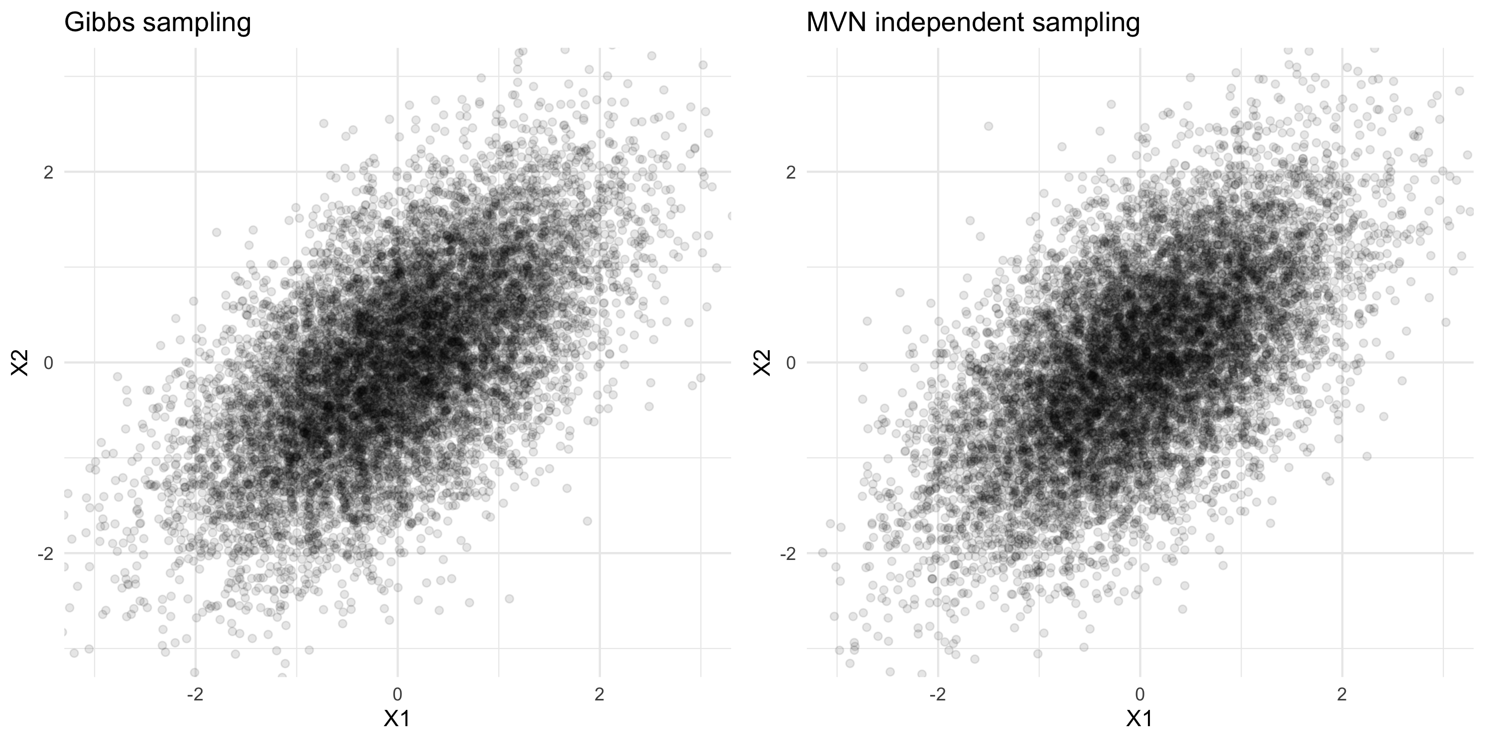
Finding p(\beta, \tau^2, \theta | Y)
We know how to get
\{ \tau^2_{(t)}, \beta_{(t)} \}_{t=1}^T \qquad \text{where} \qquad \tau^2_{(t)}, \beta_{(t)} \sim p(\beta, \tau^2 | Y, \theta)
We “know” how to get
\{ \theta_{(t)} \}_{t=1}^T \qquad \text{where} \qquad \theta_{(t)} \sim p(\theta | Y, \beta, \tau^2)
Therefore, we build a Gibbs sampler and get
\{ \tau^2_{(t)}, \beta_{(t)}, \theta_{(t)} \}_{t=1}^T \qquad \text{where} \qquad \tau^2_{(t)}, \beta_{(t)}, \theta_{(t)} \sim p(\beta, \tau^2, \theta | Y)
We learn p(\beta, \tau^2, \theta | Y) by summarizing samples from it.
Marginal posteriors:
Need samples from p(\beta | Y), p(\tau^2 | Y), p(\theta | Y)?
Just pick the element we need, e.g. extract \{ \beta_{(t)} \}_{t=1}^T from \{ \tau^2_{(t)}, \beta_{(t)}, \theta_{(t)} \}_{t=1}^T for a sample from p(\beta | Y)
With samples from p(\beta, \tau^2, \theta | Y)
One important thing we still need is p(w | Y), the posterior for the spatial process
\begin{align*} p(w | Y) &= \int p(\beta, \tau^2, \theta, w | Y) d\beta d\tau^2 d\theta \\ &= \int p(w | Y, \beta, \tau^2, \theta) p(\beta, \tau^2, \theta | Y) d\beta d\tau^2 d\theta \end{align*}
- This means that for each sample of \tau^2_{(t)}, \beta_{(t)}, \theta_{(t)}, all we need to do is independently sample from p(w | Y, \beta, \tau^2, \theta) to obtain a sample from the joint posterior.
- p(w | Y, \beta, \tau^2, \theta) is our next target
- It will be simple!
Finding p(w | Y, \beta, \tau^2, \theta)
- Before we start, take a moment to notice what we are trying to do
- We want a posterior (we condition on Y) but we take everything else as known
Prior: w | \theta \sim N(0, C_{\theta})
Model: Y = X\beta + w + \varepsilon,\quad \varepsilon \sim N(0, \tau^2 I_n)
Rewrite the model: Y^* = I_n w + \varepsilon \qquad \text{where}\quad Y^* = Y-X\beta
(full conditional) Posterior
How do we continue?
Finding p(w | Y, \beta, \tau^2, \theta)
- Before we start, take a moment to notice what we are trying to do
- We want a posterior (we condition on Y) but we take everything else as known
Prior: w | \theta \sim N(0, \tau^2 C_{\theta})
Model: Y = X\beta + w + \varepsilon,\quad \varepsilon \sim N(0, \tau^2 I_n)
Rewrite the model: Y^* = I_n w + \varepsilon \qquad \text{where}\quad Y^* = Y-X\beta
(full conditional) Posterior
This is just the usual linear regression. Here, w plays the role of \beta. It is a Gaussian model with Gaussian prior, so the posterior is Gaussian (conjugate):
\begin{align*} &w | Y, \beta, \tau^2, \theta \sim N(m_w, \tau^2 \Sigma_w)\\ &\Sigma_w^{-1} = C_{\theta}^{-1} + I_n\\ &m_w = \Sigma_w (Y - X\beta) \end{align*}
Predictions
- The last thing we are left to figure out is how to make predictions at new locations
- We know how to do that for a GP response model (How?), what about now?
- We are looking for Y(s^*) where s^* was not originally in our dataset
Y(s^*) \sim N( X(s^*)^\top \beta + w(s^*), \tau^2)
- First, note that p(w(s^*) | w, Y) = p(w(s^*) | w)
- p(w(s^*) | w) is the GP prediction as we saw it here
- With samples \tau^2_{(t)}, \beta_{(t)}, \theta_{(t)}, w_{(t)}, we just need to compute p(w(s^*) | w) and then extract from Y(s^*) \sim N( X(s^*)^\top \beta + w(s^*), \tau^2)
Why? Because:
\begin{align*} p(Y^*, w^*, w, \beta, \tau^2, \theta | Y) &= p(Y^*, w^* | Y, w, \beta, \tau^2, \theta) p(w, \beta, \tau^2, \theta | Y) \\ &= p(Y^* | w^*, Y, w, \beta, \tau^2, \theta) p(w^* | Y, w, \beta, \tau^2, \theta) p(w, \beta, \tau^2, \theta | Y) \\ &= p(Y^* | w^*, \beta, \tau^2) p(w^* | w, \theta)p(w, \beta, \tau^2, \theta | Y) \end{align*}
Back to the DAG
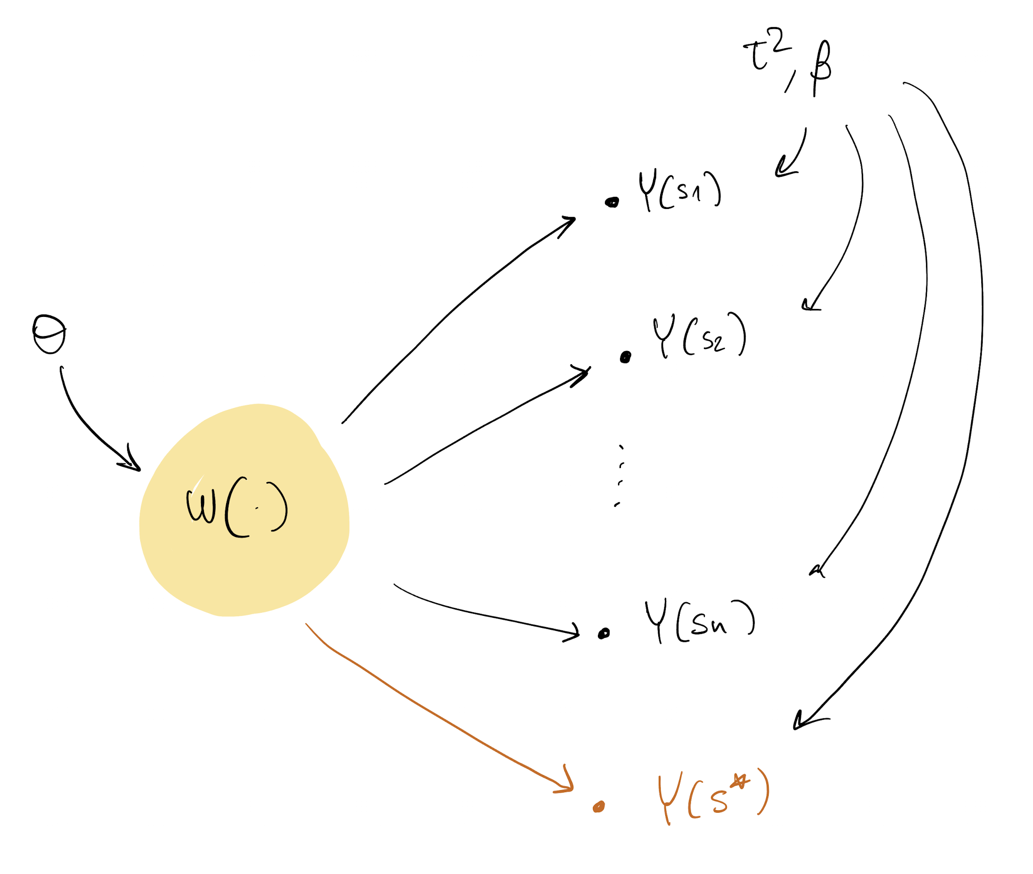
Back to the DAG
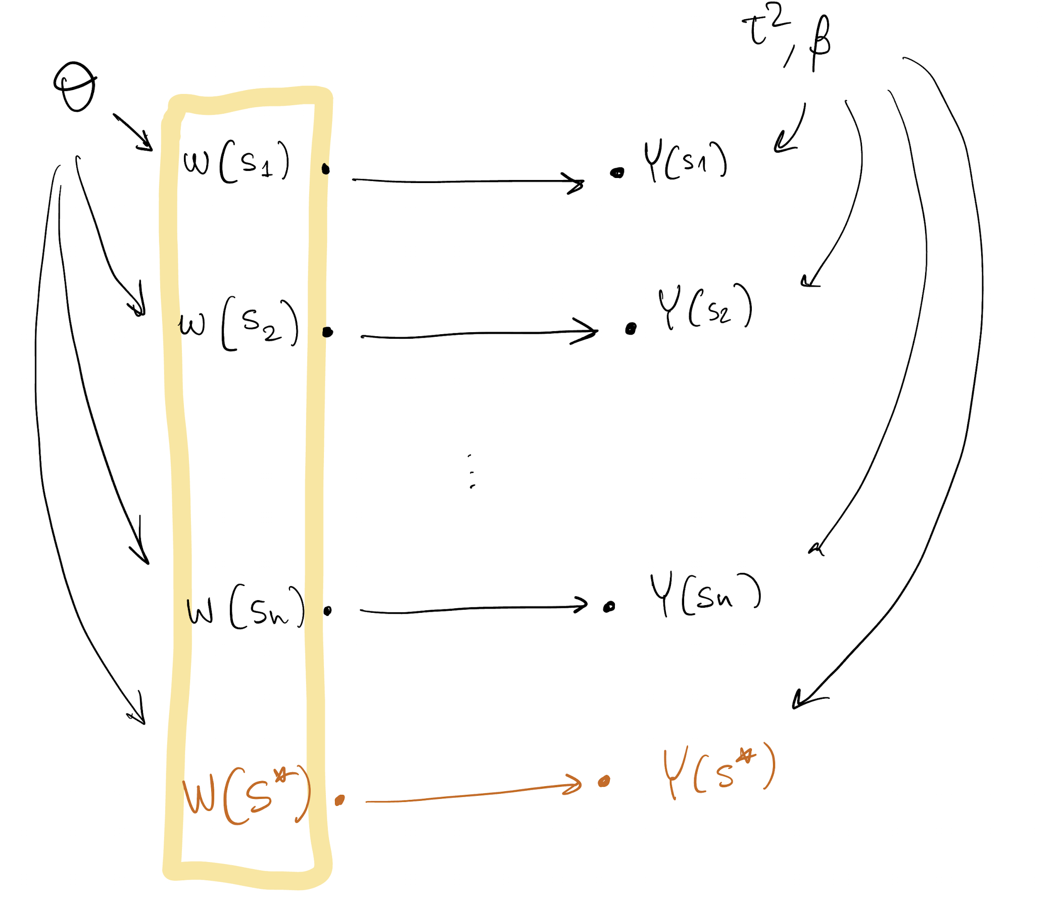
We’re done!
- We have outlined all steps for estimating parameters and making predictions
- The basic univariate linear spatial model can be extended in many ways
- Make it a latent-Gaussian model of non-Gaussian data (spatial GLMM)
- The model we have considered is also referred to as a spatially-varying intercept model
- Assume Z(s) \in \Re is a covariate not already in X(s). Then,
Y(s) = X(s) \beta + Z(s) w(s) + \varepsilon(s) is a spatially-varying coefficient (SVC) model. The regression coefficient that explains how Z(s) is associated to Y(s) is a spatial process (basically, we can draw a map of it) rather than a constant
But we are not done!!!
We have not explained how we are getting samples
\{ \theta_{(t)} \}_{t=1}^T \qquad \text{where} \qquad \theta_{(t)} \sim p(\theta | Y, \beta, \tau^2)
For that, we need to outline the Metropolis-Hastings algorithm.
Metropolis-Hastings algorithm
- Goal: obtain samples from a target density p(x)
- Idea: make a Markov chain that has p(x) as its stationary distribution
Iteration t of the MH algorithm
- Given the current value x_{(t-1)}, propose a new value x^* by sampling it from density q(\cdot | x_{(t-1)})
- Compute (by evaluating the densities) \alpha = \frac{p(x^*)}{p(x_{(t-1)})} \frac{q(x_{(t-1)}| x^*)}{q(x^* | x_{(t-1)})}
- Accept and therefore set x_{(t)} = x^* with probability \min\{1, \alpha\}
- For example, sample U \sim U(0,1) and accept if U < \alpha, reject otherwise
- We have built a Markov chain, and it can be shown to converge to p(\cdot)
- Output: (correlated) samples \{ x_{(t)} \}_{t=1}^T
In our case
- Our target is p(\theta | Y, \beta, \tau^2) \propto p(Y | \theta, \beta, \tau^2) p(\theta)
- Because we are taking ratios of this target, the normalizing constant cancels out
- This is very convenient: MH works even if we can only evaluate the target density up to a proportionality constant
Metropolis-Hastings algorithm
- Goal: obtain samples from p(\theta | Y, \beta, \tau^2) \propto p(Y | \theta, \beta, \tau^2) p(\theta)
- Idea: make a Markov chain that has p(Y | \theta, \beta, \tau^2) p(\theta) as its stationary distribution
Iteration t of the MH algorithm
Given the current value \theta_{(t-1)}, propose a new value \theta^* by sampling it from density q(\cdot | \theta_{(t-1)})
Compute (by evaluating the densities) \alpha = \frac{p(Y | \theta^*, \beta, \tau^2) p(\theta^*)}{p(Y | \theta_{(t-1)}, \beta, \tau^2) p(\theta_{(t-1)})} \frac{q(\theta_{(t-1)}| \theta^*)}{q(\theta^* | \theta_{(t-1)})}
Accept and therefore set \theta_{(t)} = \theta^* with probability \min\{1, \alpha\}
For example, sample U \sim U(0,1) and accept if U < \alpha, reject otherwise
Output: (correlated) samples \{ \theta_{(t)} \}_{t=1}^T from p(\theta | Y, \beta, \tau^2)
Metropolis-Hastings algorithm & Gibbs samplers
- A Gibbs sampler assumes we can sample from all the full conditional distributions
- We would then alternate sampling from each of them to obtain a correlated sample from the joint posterior
- If even one of the full conditionals is not available, we can replace that step with a Metropolis-Hastings step
- The resulting Metropolis-within-Gibbs algorithm is one of the most important algorithms in Bayesian statistics because of its extremely wide applicability
- The Gibbs sampler itself is a special case of Metropolis-Hastings
- Many generalizations of Metropolis-Hastings (adaptive MH, Hamiltonian MC, …)
Back to finding p(\beta, \tau^2, \theta | Y)
We use a conditionally conjugate step to get
\{ \tau^2_{(t)}, \beta_{(t)} \}_{t=1}^T \qquad \text{where} \qquad \tau^2_{(t)}, \beta_{(t)} \sim p(\beta, \tau^2 | Y, \theta)
We use Metropolis-Hastings to get
\{ \theta_{(t)} \}_{t=1}^T \qquad \text{where} \qquad \theta_{(t)} \sim p(\theta | Y, \beta, \tau^2)
Therefore, we build a Metropolis-within-Gibbs sampler and get
\{ \tau^2_{(t)}, \beta_{(t)}, \theta_{(t)} \}_{t=1}^T \qquad \text{where} \qquad \tau^2_{(t)}, \beta_{(t)}, \theta_{(t)} \sim p(\beta, \tau^2, \theta | Y)
We learn p(\beta, \tau^2, \theta | Y) by summarizing samples from it.
Alternative sampling algorithms
- In the previous discussion, we have marginalized out w
- This is convenient because w is high dimensional
- The “remaining” joint posterior is lower dimensional
- Lower dimension = easier to explore and learn
- We could also integrate out \beta (R package
spBayesdoes this)
Non-marginalized sampler
What if we do not integrate out w?
We are then looking at the joint posterior p(w, \beta, \tau^2, \theta | Y)
Here, a Gibbs sampler (with a Metropolis step) works this way:
- Sample from p(\tau^2 | Y, w, \beta, \theta)
- Sample from p(w | Y, \beta, \tau^2, \theta)
- Sample from p(\beta | Y, w, \tau^2, \theta)
- Update \theta with a Metropolis step targeting p(\theta | Y, w, \tau^2, \beta)
Non-marginalized sampler
What if we do not integrate out w?
We are then looking at the joint posterior p(w, \beta, \tau^2, \theta | Y)
Here, a Gibbs sampler (with a Metropolis step) works this way:
- Sample from p(\tau^2 | Y, w, \beta, \theta) = p(\tau^2 | Y, w, \beta) why?
- Sample from p(w | Y, \beta, \tau^2, \theta)
- Sample from p(\beta | Y, w, \tau^2, \theta) = p(\beta | Y, w, \tau^2) why?
- Update \theta with a Metropolis step targeting p(\theta | Y, w, \tau^2, \beta) = p(\theta | w) why?
Non-marginalized sampler
What if we do not integrate out w?
We are then looking at the joint posterior p(w, \beta, \tau^2, \theta | Y)
Here, a Gibbs sampler (with a Metropolis step) works this way:
- Sample from p(\tau^2 | Y, w, \beta)
- Sample from p(w | Y, \beta, \tau^2, \theta)
- Sample from p(\beta | Y, w, \tau^2)
- Update \theta with a Metropolis step targeting p(\theta | w) \propto p(w | \theta) p(\theta) what is p(w | \theta)?
Non-marginalized sampler, step 1
- Sample from p(\tau^2 | Y, w, \beta)
- We condition on everything else, so Y^* = Y-X\beta - w can be computed
- Treat Y^* as the dataset
- Then the prior-model pair is
\begin{align*} \tau^2 &\sim Inv.G(a_{\tau}, b_{\tau})\\ Y^* &\sim N(0, \tau^2 I_n) \end{align*}
- How do we find the (full conditional) posterior in this case?
Non-marginalized sampler, step 1
- Sample from p(\tau^2 | Y, w, \beta)
- We condition on everything else, so Y^* = Y-X\beta - w can be computed
- Treat Y^* as the dataset
- Then the prior-model pair is
\begin{align*} \tau^2 &\sim Inv.G(a_{\tau}, b_{\tau})\\ Y^* &\sim N(0, \tau^2 I_n) \end{align*}
- In the usual linear regression model, drop everything related to \beta
- Inverse Gamma full conditional
Non-marginalized sampler, step 2
- Sample from p(w | Y, \beta, \tau^2, \theta)
- Treat Y^* = Y - X\beta as the dataset
- Then the prior-model pair is
\begin{align*} w &\sim N(0, C_{\theta})\\ Y^* &\sim N(I_n w, \tau^2 I_n) \end{align*}
- How do we find the (full conditional) posterior in this case?
Non-marginalized sampler, step 2
- Sample from p(w | Y, \beta, \tau^2, \theta)
- Treat Y^* = Y - X\beta as the dataset
- Then the prior-model pair is
\begin{align*} w &\sim N(0, C_{\theta})\\ Y^* &\sim N(I_n w, \tau^2 I_n) \end{align*}
- This is a regression model with known error variance
- Gaussian prior, Gaussian model, therefore Gaussian posterior
- p(w | Y, \beta, \tau^2, \theta) = N(w; \mu_w, \Sigma_w) where
\begin{align*} \Sigma_w^{-1} &= C_{\theta}^{-1} + 1/\tau^2\\ \mu_w &= \Sigma_w (Y - X\beta)/\tau^2 \end{align*}
Non-marginalized sampler, step 3
- Sample from p(\beta | Y, w, \tau^2)
- Treat Y^* = Y - w as the dataset
- Then the prior-model pair is
\begin{align*} \beta &\sim N(0, V)\\ Y^* &\sim N(X\beta, \tau^2 I_n) \end{align*}
- How do we find the (full conditional) posterior in this case?
Non-marginalized sampler, step 3
- Sample from p(\beta | Y, w, \tau^2)
- Treat Y^* = Y - w as the dataset
- Then the prior-model pair is
\begin{align*} \beta &\sim N(0, V)\\ Y^* &\sim N(X\beta, \tau^2 I_n) \end{align*}
- This is a regression model with known error variance
- Gaussian prior, Gaussian model, therefore Gaussian posterior
- p(\beta | Y, w, \tau^2, \theta) = N(\beta; \mu_{\beta}, \Sigma_{\beta}) where
\begin{align*} \Sigma_{\beta}^{-1} &= V^{-1} X^\top X/\tau^2\\ \mu_{\beta} &= \Sigma_{\beta} X^\top (Y - w)/\tau^2 \end{align*}
Non-marginalized sampler, step 4
- Update p(\theta | w) \propto p(w | \theta) p(\theta)
- p(w | \theta) = N(w; 0, C_{\theta})
Alternative methods
Because Y = X\beta + w + \varepsilon can be written as Y = \begin{bmatrix} X & I_n\end{bmatrix} \begin{bmatrix} \beta \\ w \end{bmatrix} + \varepsilon
We can call X^* = \begin{bmatrix} X & I_n\end{bmatrix} and \beta^* = \begin{bmatrix} \beta \\ w \end{bmatrix} and then update as a block via
p(\beta^* | Y, \tau^2, \theta) = N(\beta^*; \mu_{\beta^*}, \Sigma_{\beta^*})
- \Sigma_{\beta^*}^{-1} = V_{\beta^*}^{-1} + X^{*^\top} X^*/\tau^2
- \mu_{\beta^*} = \Sigma_{\beta^*} X^{*^\top} Y/\tau^2
- Once again, this follows from the linear regression posterior we saw in the preliminaries
Using package spBayes for spatial linear regression with latent GPs
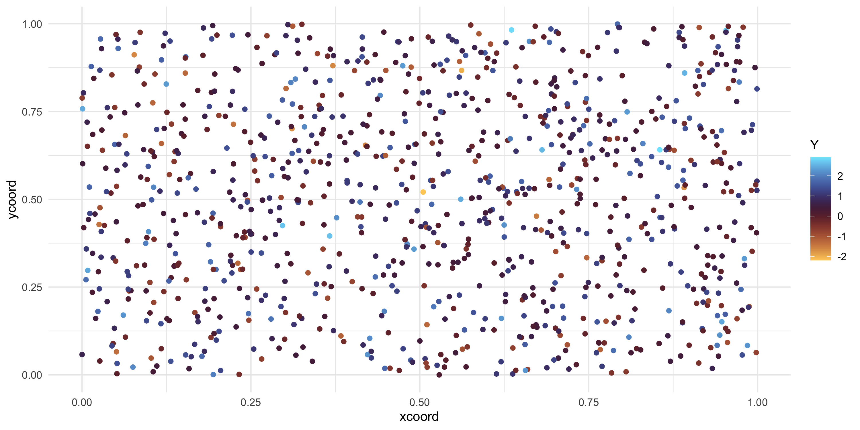
Using package spBayes for spatial linear regression with latent GPs
- First, specify how we want to set things up.
- The model we are implementing is
Y = X\beta + w + \varepsilon, \qquad \text{where}\quad \varepsilon \sim N(0, \tau^2 I_n)
Priors:
- \beta \sim N(0, 10^3 I_p) where p is the number of columns of X
- w(\cdot) \sim GP(0, C_{\sigma^2, \phi}(\cdot)) and we let C_{\sigma^2, \phi}(s, s') = \sigma^2 \exp\{ -\phi \| s-s' \| \}
- \tau^2 \sim Inv.G(2, 0.1) and \sigma^2 \sim Inv.G(2,2)
- \phi \sim U(3, 30). It is common to let \phi have a uniform prior where the range of possible values is set to give “reasonable” spatial dependence
library(spBayes)

n.samples <- 2000

starting <- list("phi"=3/0.5, "sigma.sq"=50, "tau.sq"=1)
tuning <- list("phi"=0.1, "sigma.sq"=0.1, "tau.sq"=0.1)

priors <- list("beta.Norm"=list(rep(0,ncol(X)), diag(1000,ncol(X))),
                 "phi.Unif"=c(3/1, 3/0.1), "sigma.sq.IG"=c(2, 2),
                 "tau.sq.IG"=c(2, 0.1))

cov.model <- "exponential"
Using package spBayes for spatial linear regression with latent GPs
We fit the GP regression model in 2 steps
Using package spBayes for spatial linear regression with latent GPs
- We chose to run MCMC for 2000 iterations
- If we are satisfied with convergence, we drop some initial samples (burn-in period) because they are likely not sampled at convergence
- Recall with MCMC we get correlated samples from the joint posterior after reaching convergence
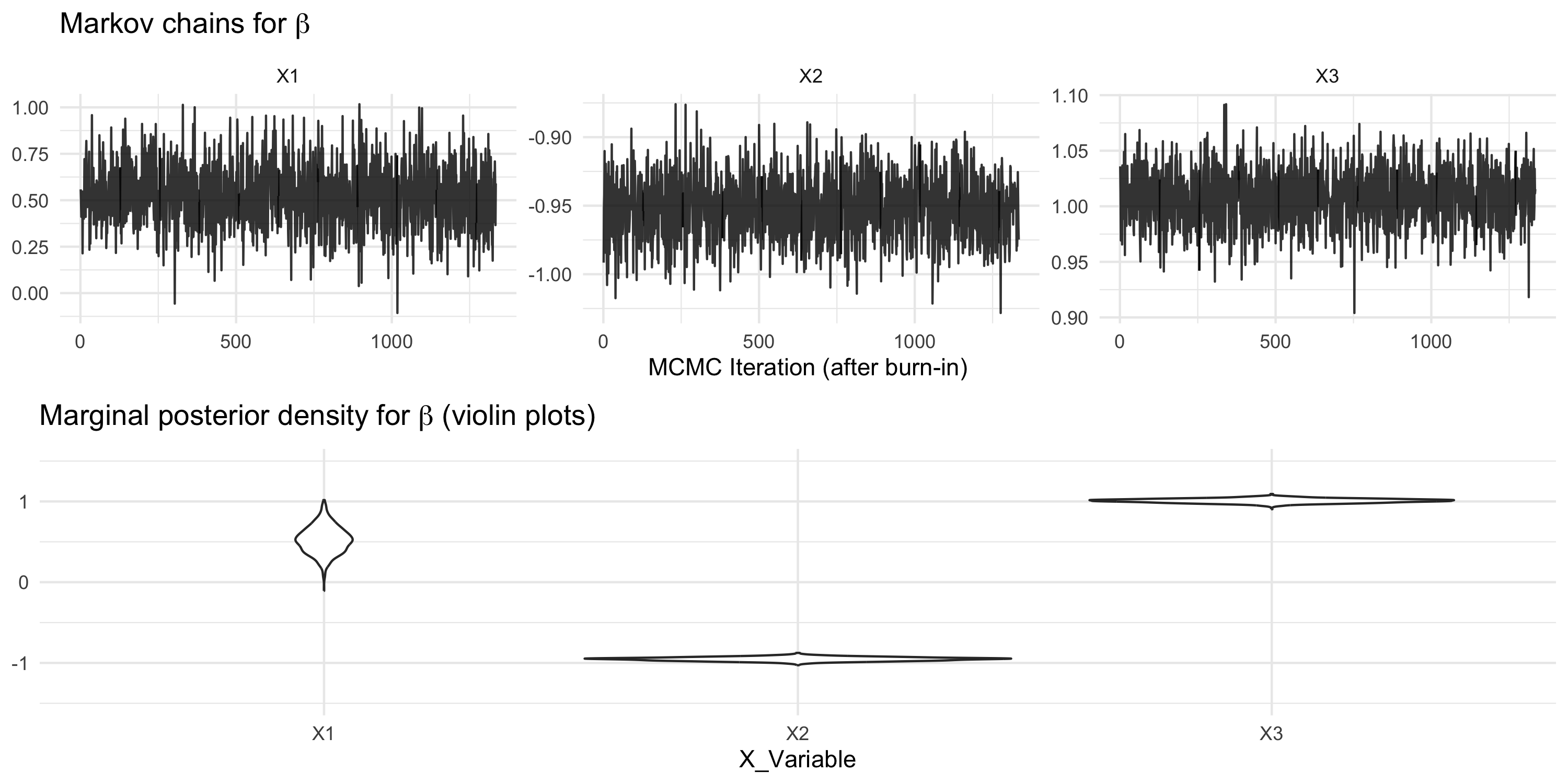
Using package spBayes for spatial linear regression with latent GPs
spBayescallsthetathe vector of (\sigma^2, \tau^2, \phi)- In this example, the MCMC chains look poor
- All chains mix poorly, or in other terms they show high autocorrelation
- Inference based on these chains should not be trusted
- We need to improve MCMC tuning and possibly run the Markov chain longer
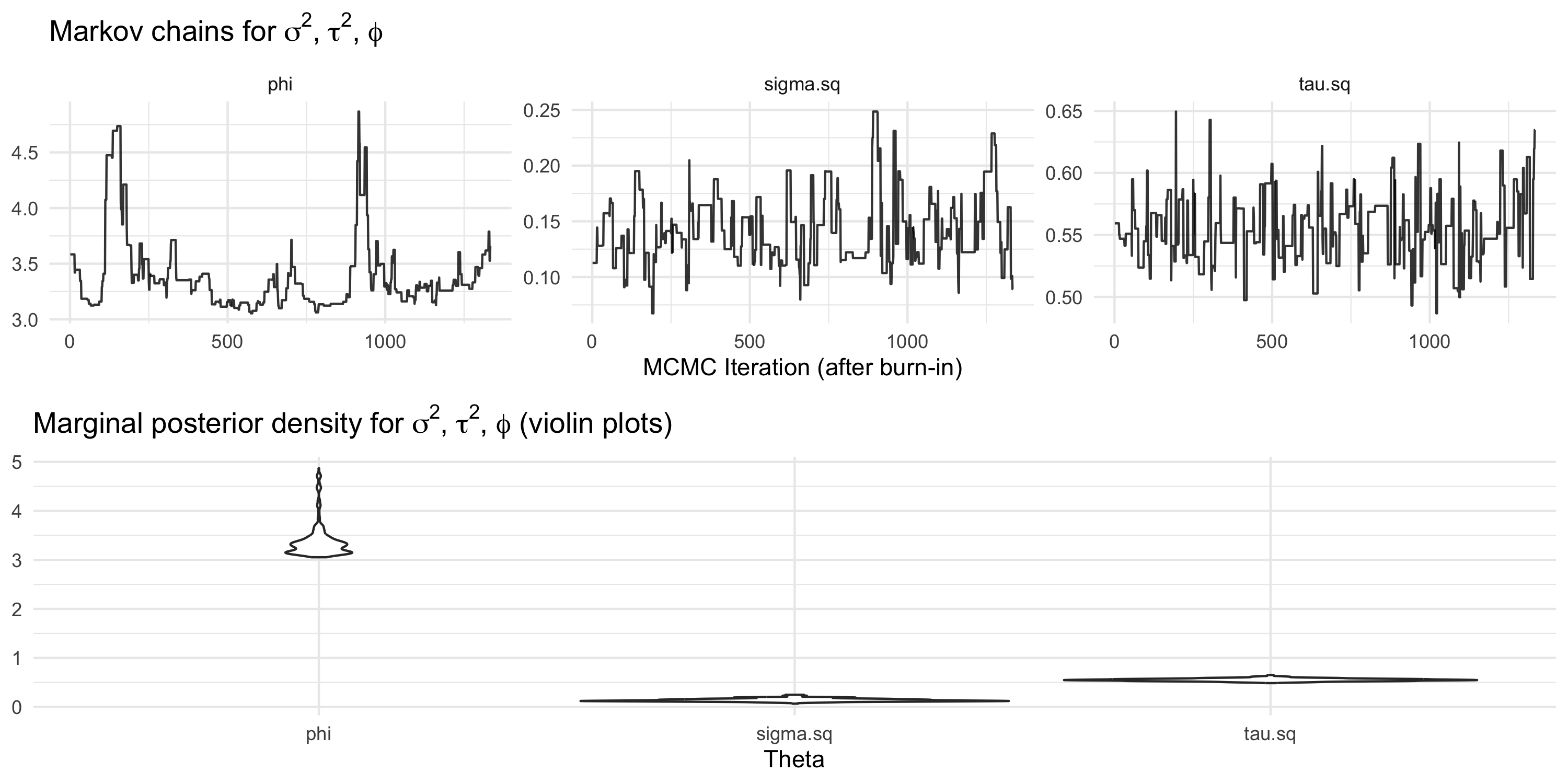
Using package spBayes for spatial linear regression with latent GPs
- At each step, a new proposed value for \phi is generated
tuning <- list("phi"=0.1, "sigma.sq"=0.1, "tau.sq"=0.1)sets the standard deviation of the proposal forphito0.1- In other words, this determines the jump size
- If the jump is too big, the proposal will probably get rejected
- In our case: 16.4% acceptance rate
- We target an acceptance rate of about 24% so we should lower
tuning$phi
Using package spBayes for spatial linear regression with latent GPs
- Let’s take the previous MCMC run (even though we did not like it too much)
- We can now predict at a grid of locations
----------------------------------------
    General model description
----------------------------------------
Model fit with 1000 observations.

Prediction at 900 locations.

Number of covariates 3 (including intercept if specified).

Using the exponential spatial correlation model.

-------------------------------------------------
        Sampling
-------------------------------------------------
Sampled: 100 of 2000, 4.95%
Sampled: 200 of 2000, 9.95%
Sampled: 300 of 2000, 14.95%
Sampled: 400 of 2000, 19.95%
Sampled: 500 of 2000, 24.95%
Sampled: 600 of 2000, 29.95%
Sampled: 700 of 2000, 34.95%
Sampled: 800 of 2000, 39.95%
Sampled: 900 of 2000, 44.95%
Sampled: 1000 of 2000, 49.95%
Sampled: 1100 of 2000, 54.95%
Sampled: 1200 of 2000, 59.95%
Sampled: 1300 of 2000, 64.95%
Sampled: 1400 of 2000, 69.95%
Sampled: 1500 of 2000, 74.95%
Sampled: 1600 of 2000, 79.95%
Sampled: 1700 of 2000, 84.95%
Sampled: 1800 of 2000, 89.95%
Sampled: 1900 of 2000, 94.95%
Sampled: 2000 of 2000, 99.95%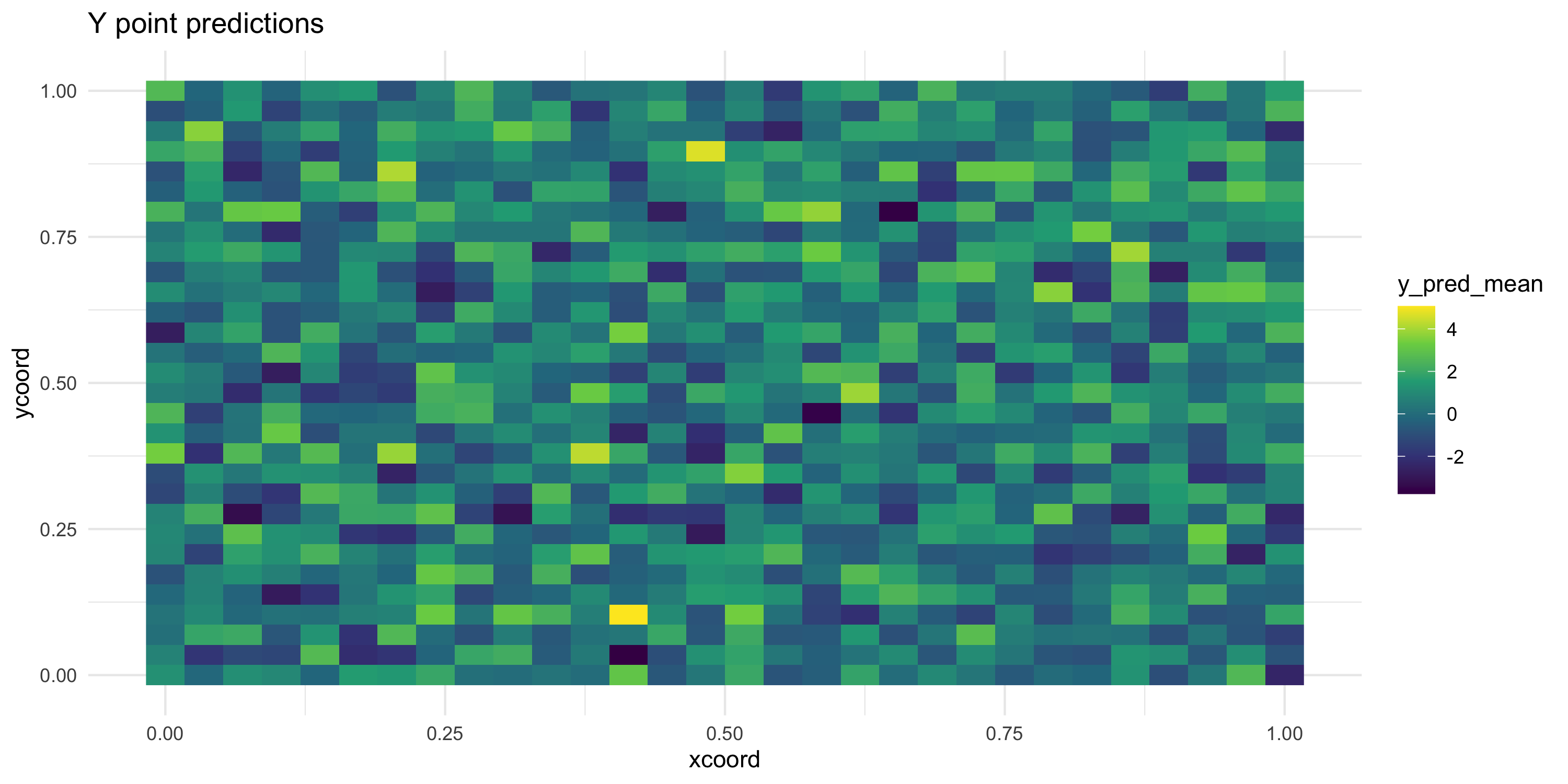
Using package spBayes for spatial linear regression with latent GPs
- Calculate residuals from the model fit
w_post <- model_fit$p.w.recover.samples
b_post <- model_fit$p.beta.recover.samples
XB_post <- X %*% t(b_post)
XBW_mean <- (XB_post + w_post) %>% apply(1, mean)
model_residual <- Y - XBW_mean

df <- df %>% mutate(residual = model_residual)
residual_map <- ggplot(df, aes(xcoord, ycoord, color=residual)) +
  geom_point() +
  scale_color_viridis_c() +
  theme_minimal() +
  ggtitle("Residual")

sv <- df %>% with(geoR::variog(data = residual, coords = cbind(xcoord, ycoord), messages=FALSE))

sv_df <- data.frame(dists = sv$u, variogram = sv$v, npairs = sv$n, sd = sv$sd)
sv_plot <- ggplot(sv_df, aes(x=dists, y=variogram)) + geom_point(size=2, shape=8) +
  theme_minimal()

grid.arrange(residual_map, sv_plot, nrow=1)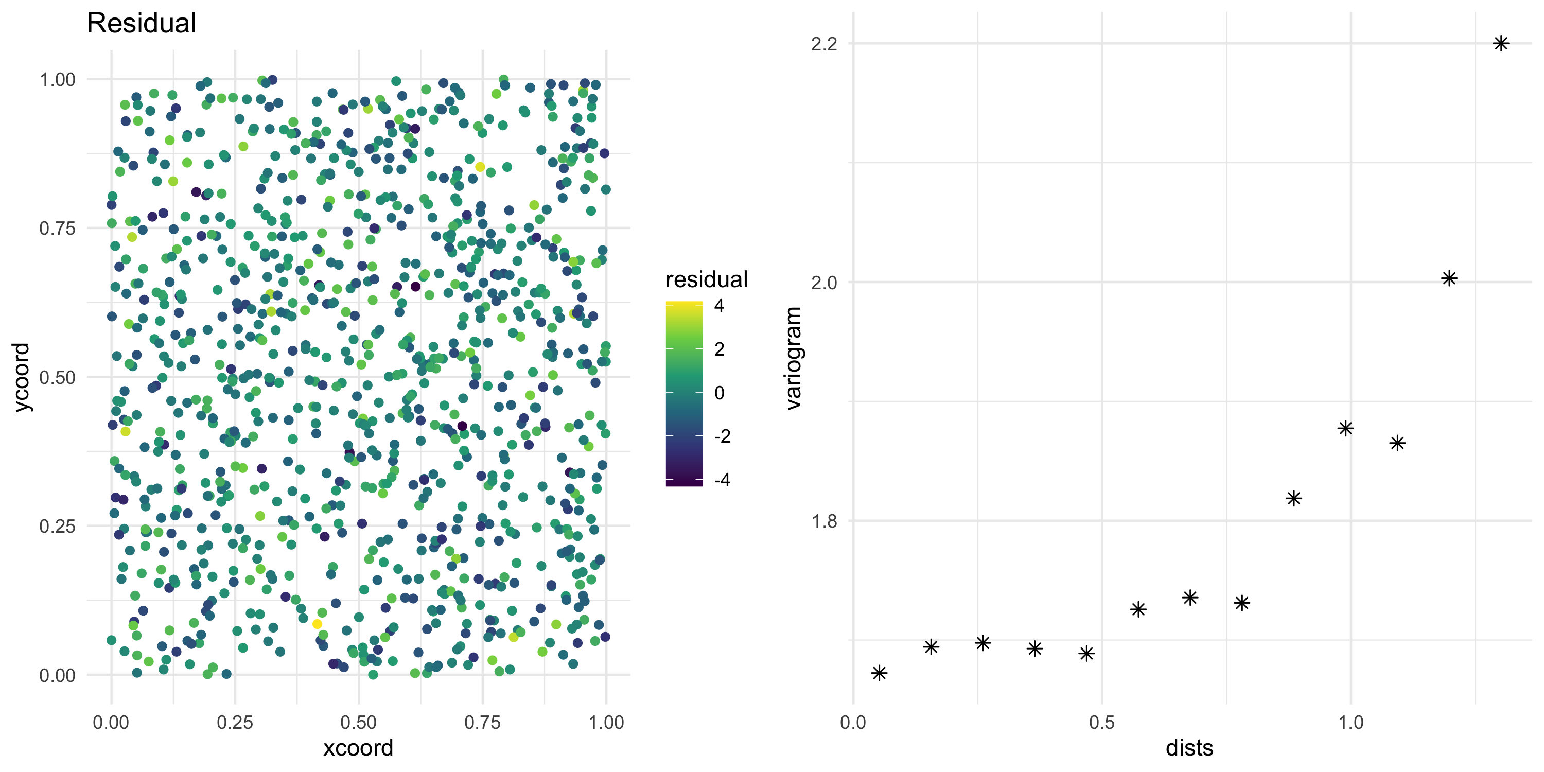
Why does spBayes need two steps
Priors:
- \tau^2 \sim Inv.G(a_{\tau}, b_{\tau})
- \beta \sim N(0, \tau^2 V)
- s^2 \sim Inv.G(a_{s}, b_s)
- \phi \sim U(l_{\phi}, u_{\phi})
- w(\cdot) \sim GP(0, C_{s, \phi}(\cdot)) where C_{s, \phi}(s, s') = \sigma^2 \exp\{ -\phi \| s-s' \| \}
Model:
Y(s) = X(s)^\top \beta + w(s) + \varepsilon(s),\ \text{where}\ \varepsilon(s) \sim N(0, \tau^2) \quad \text{(iid)} In vector form: Y = X\beta + w + \varepsilon, where \varepsilon \sim N(0, \tau^2 I_n).
Marginalized model:
- In addition to integrating out w as we have seen before, we can also do that with \beta
- In
spBayes, this is the marginal model that is fit via MCMC
Y | \tau^2, s^2, \phi \sim N(0, \tau^2 (X V X^\top + I_n) + C_{\sigma^2, \phi})
Why does spBayes need two steps
Marginalized model:
- In addition to integrating out w as we have seen before, we can also do that with \beta
- In
spBayes, this is the marginal model that is fit via MCMC
Y | \tau^2, s^2, \phi \sim N(0, \tau^2 (X V X^\top + I_n) + C_{\sigma^2, \phi})
- It is possible to update \tau^2 via a Gibbs step or jointly with \phi and \sigma^2 as a Metropolis update
- The Metropolis-Hastings algorithm targets the posterior p(\tau^2, \sigma^2, \phi | Y) \propto p(Y | \tau^2, \sigma^2, \phi) p(\tau^2, \sigma^2, \phi)
- Once we have samples from p(\tau^2, \sigma^2, \phi | Y) we can sample from p(\beta | Y, \tau^2, \sigma^2, \phi)
- Once we have samples from p(\tau^2, \sigma^2, \phi | Y) we can sample from p(w | Y, \tau^2, \sigma^2, \phi)
- Both of these steps are performed in
spRecover
Moving forward
spBayes::spLMfits a GP regression model- Computations take a considerable amount of time for n=1000
- Datasets with n=10000 or larger are quite common
- Let’s see what happens with
spLMat increasing sample sizes
Moving forward
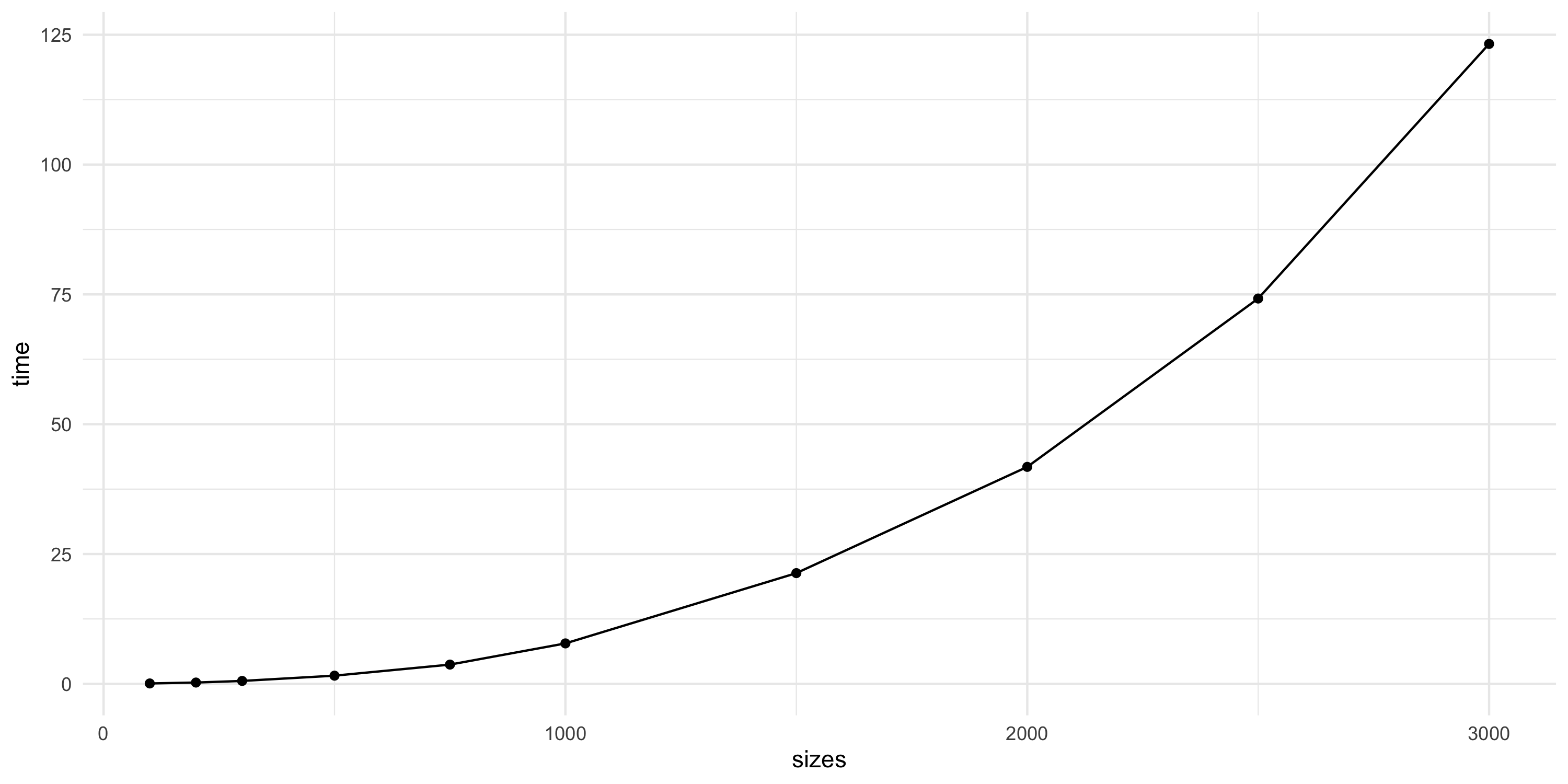
- Things do not look promising
- Next, we will look into why this is the performance profile we get
- We will then consider some solutions to the scalability problem