Quick review of preliminaries
Spatial Statistics - BIOSTAT 696/896
Michele Peruzzi
University of Michigan
Random variables and random vectors
- Real-valued function defined on outcome of experiment Y : \Omega \to \Re
- Example: Bernoulli r.v. represents coin toss with values \{0,1\} each corresponding to \Omega = \{ H, T \}
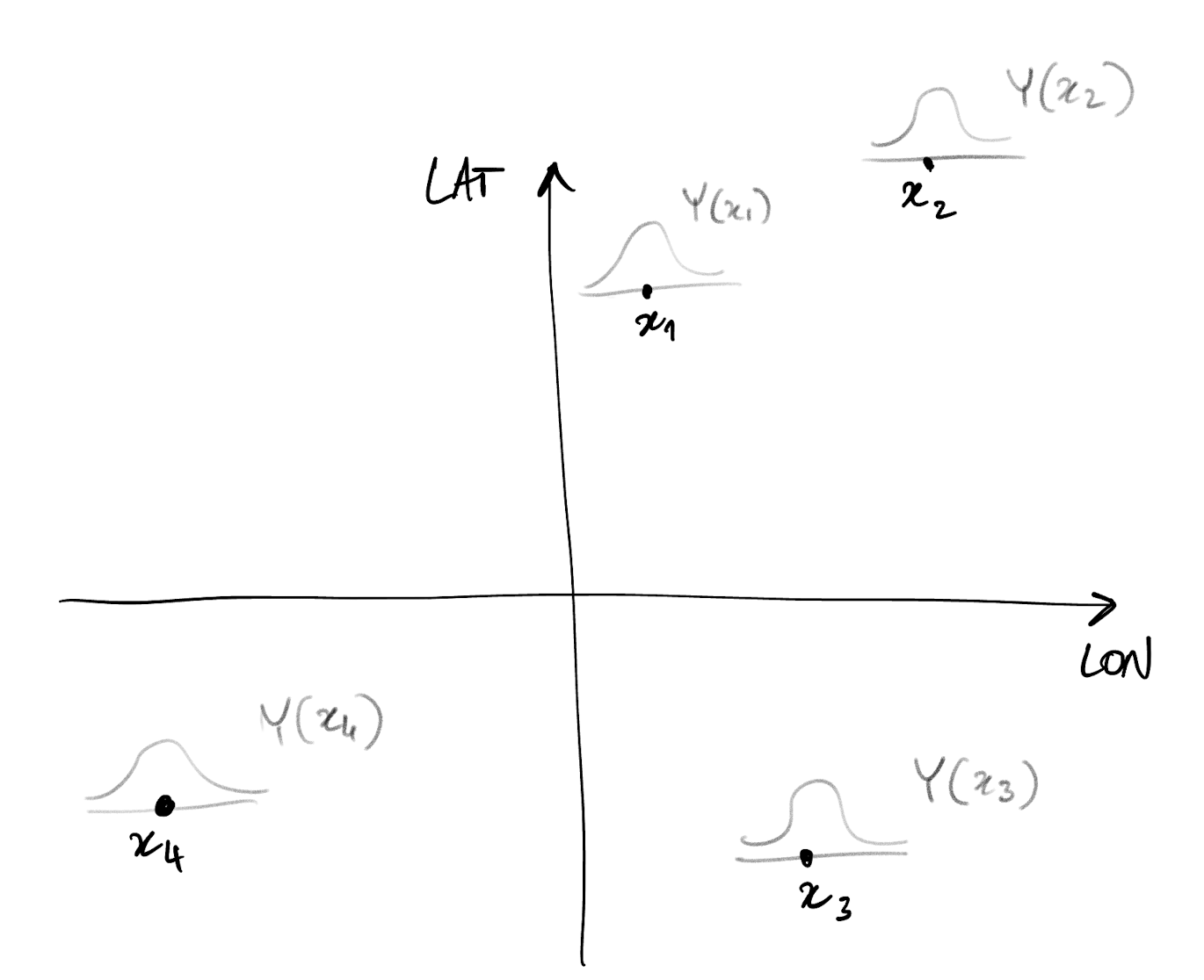
- With spatial data, we have one random variable at each domain location
- In other words, we have a spatial index
- Example: Y(x) is the random variable at location x
- When we speak of multivariate spatial data, we mean Y(x) is a random vector
Random variables and random vectors
- With spatial data, we have one random variable at each domain location
- In other words, we have a spatial index
- Example: Y(x) is the random variable at location x
- Our aim is to model the dependence structure of any given set of such spatially-indexed random variables
Expectation, covariance, conditional expectation
- E[Y] = \int y f(y)dy where f(y) is the probability density function of Y
- Cov[X, Y] = E[X - E[X]]E[Y - E[Y]] = E[XY] - E[X]E[Y]
- Cov is a linear operator
- Conditional expectation E[Y|X] = \int y f_{Y|X}(y|x) is the expectation of the random variable Y | X = x
- Cov[X, Y] = E[Cov[X,Y | Z]] + Cov[E[X|Z], E[Y|Z]]
- In particular Var[X] = E[Var[X|Y]] + Var[E[X|Y]]
Joint density of a collection of random variables
- Suppose we have two (continuous) random variables X and Y
- Denote their joint probability density is f(X,Y)
- We can write f(X,Y) = f(X) f(Y | X) = f(Y) f(X | Y) where f(X) is the marginal density of X
- Why is this useful? Sometimes, specifying f(X,Y) directly is difficult
- Easier to specify f(X) (or f(Y)) and then the conditional density f(Y | X) (or f(X|Y))
- i.e. model X, then model Y for every given value of X
- More in general, with X,Y,Z, we can write f(X,Y,Z) = f(X) f(Y|X) f(Z|X,Y)
- For a set of n variables, f(X_1, \dots, X_n) = f(X_1) f(X_2 | X_1) \dots f(X_n | X_1, \dots X_{n-1})
Graphical models
- Suppose you are given a collection of random variables
- Describing their joint distribution may be difficult
- Problem may be simplified by looking at pairs of variables. Are they “related”?
- So, suppose you are given pairwise “dependence” information
- Draw one node for each random variable
- Draw one edge between each pair of dependent (ie, related) random variables
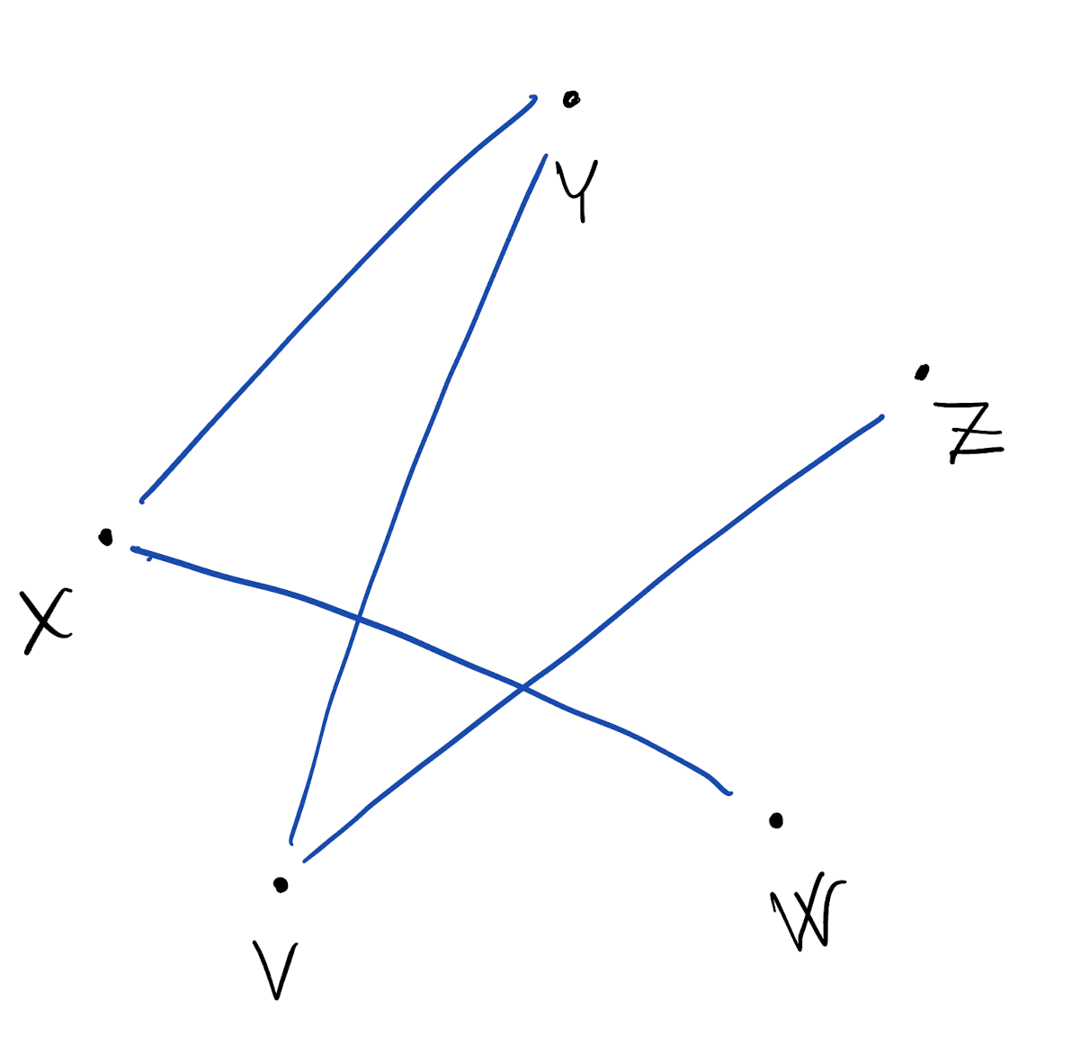
Graphical models: undirected graphs
- We can then write the resulting joint density as: f(X,Y,Z,V,W) = \frac{1}{c} f(X|W,Y) f(Y|X,V) f(Z|V) f(V|Y,Z) f(W|X) where c is an unknown normalizing constant
- We are modeling conditional independence
- The graphical model helps us conceptually in defining f(X,Y,Z,V,W) which is a complex object to deal with
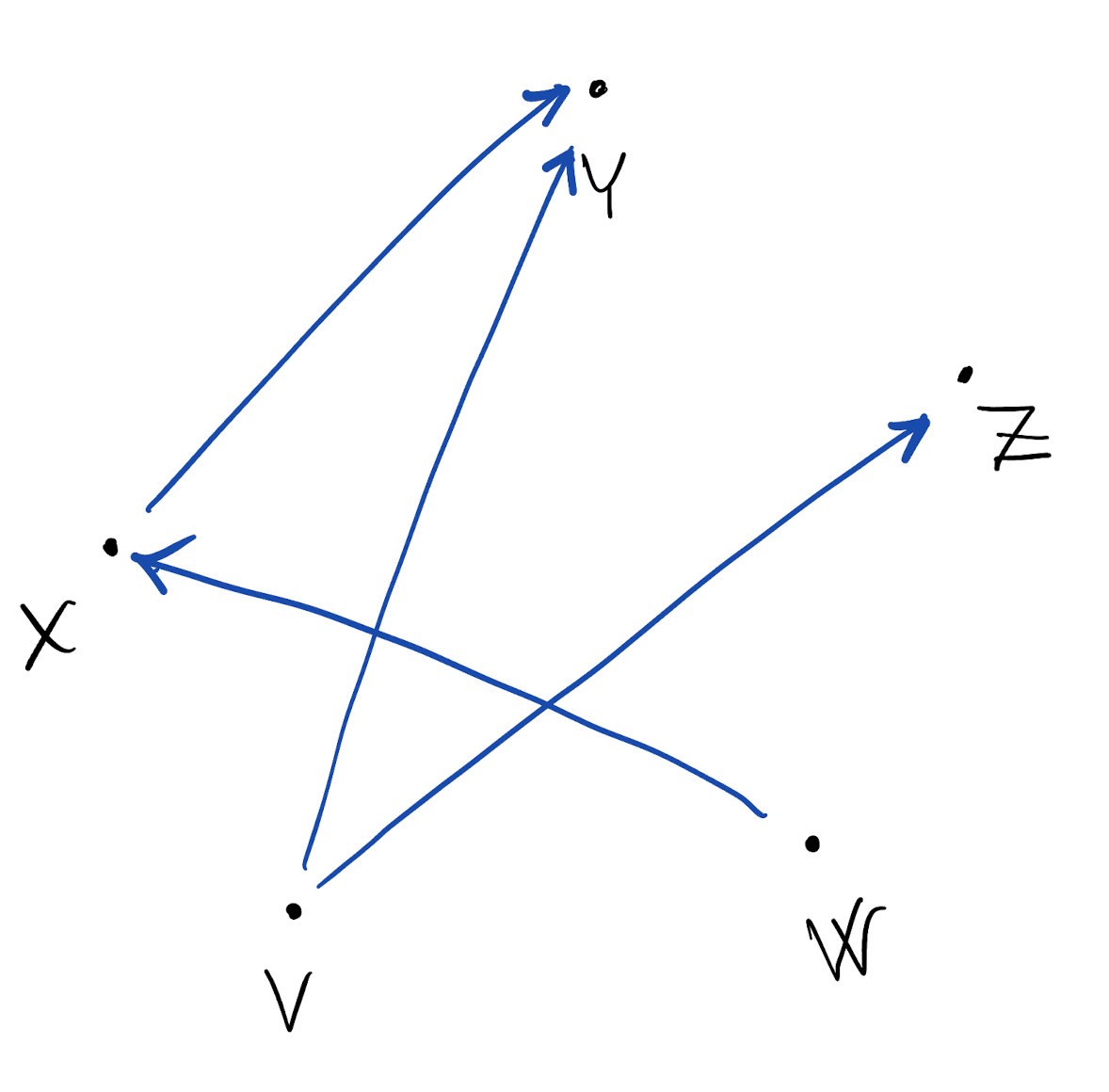
Graphical models: directed acyclic graphs (DAG)
- We can go one step further and consider a special case of graphical model
- If random variable X “explains” Y (i.e. changes in Y can be attributed to changes in X) then we represent the dependence with a directed edge X \to Y
- Remember this is a model, i.e. a representation of reality based on what we think is reasonable
- Of particular interest is when all edges are directed, and no cycles can be found
- Acyclicity: we can never start from a node, follow the “arrows”, and return to the same node
- The graphical model we obtain is a directed acyclic graph, also called a Bayesian network
Graphical models: directed acyclic graphs (DAG)
- Useful property of DAGs is that we get f(X,Y,Z,V,W) = f(X|W) f(Y|X,V) f(Z|V) f(V) f(W)
- Notice there is no normalizing constant
- We say that the joint density factorizes according to the given DAG
Bayesian paradigm
- Model everything as a random variable/vector
- Make assumptions about conditional independence between all variables
- A Bayesian (hierarchical) model can be represented as a DAG
- (this is why DAGs are also called Bayesian networks)
- This is a model for the joint probability of all variables, including the data
- Interest is in finding the conditional probability of all unknowns given the data
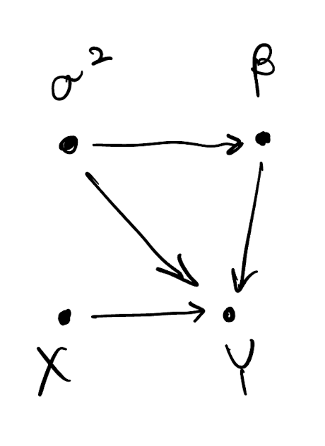
Bayesian paradigm: linear regression example
\sigma^2 \sim Inv.G(a,b) \beta \sim N(m_{\beta}, \sigma^2 V_{\beta}) Y = X \beta + \varepsilon, \text{ where } \varepsilon \sim N(0, \sigma^2 I_n) Equivalently, Y \sim N(X \beta, \sigma^2 I_n).
Bayesian paradigm: linear regression example
- We typically always condition on the covariates (X) so we need not explicitly assign them a probability model
- The joint density of all variables factorizes according to the DAG p(\sigma^2, \beta, Y) = p(\sigma^2) p(\beta | \sigma^2) p(Y | \sigma^2, \beta)
Prior, posterior, predictive distributions
- Prior distribution: the assumed marginal density of the model parameters (eg, p(\sigma^2, \beta) = Inv.G(\sigma^2; a,b) N(\beta; m_{\beta}, \sigma^2 V_{\beta}))
- Probability model/likelihood: the assumed cond. density of the data, given the parameters (eg, p(Y | \beta, \sigma^2) = N(y; X\beta, \sigma^2 V_y))
- Typically, V_y = I_n the identity matrix, but the more general case is useful
- Posterior distribution: the implied cond. density of the model parameters given the data (eg, p(\beta, \sigma^2 | Y))
- Predictive distribution: the implied cond. density of new data, given old data: p(Y^{\text{new}}| Y) = \int p(Y^{\text{new}}| Y, \beta, \sigma^2) p(\beta, \sigma^2 | Y) d\beta d\sigma^2
Bayes theorem:
P(A | B) = \frac{P(A) P(B|A)}{P(B)} Bayesian linear regression: p(\sigma^2, \beta | Y) = \frac{ p(\sigma^2, \beta) p(Y | \sigma^2, \beta) }{p(Y)} \propto p(\sigma^2, \beta) p(Y | \sigma^2, \beta)
Bayesian regression with conjugate priors
- If p(\sigma^2, \beta) is Normal-Inverse Gamma and p(Y|\beta,\sigma^2) is Normal, then p(\sigma^2, \beta | Y) is again Normal-Inverse Gamma
- Because prior and posterior belong to the same family, they are a conjugate pair
- Let p(\sigma^2, \beta) = Inv.G(\sigma^2; a,b) N(\beta; m_{\beta}, \sigma^2 V_{\beta})
- Let p(Y | \beta, \sigma^2) = N(y; X\beta, \sigma^2 V_y)
- Then the posterior is p(\sigma^2, \beta | Y) = Inv.G(\sigma^2; a^*,b^*) N(\beta; m_{\beta}^*, \sigma^2 V_{\beta}^*) where we just need to compute the updated parameters V_{\beta}^* = (V_{\beta}^{-1} + X^T V_y^{-1} X)^{-1} m_{\beta}^* = V_{\beta}^*(V_{\beta}^{-1}m_{\beta} + X^T V_y^{-1} y) a^* = a + n/2 \quad\text{and}\quad b^* = b + \frac{1}{2}(m_{\beta}^T V_{\beta}^{-1} m_{\beta} + y^TV_y^{-1} y - m_{\beta}^* V_{\beta}^{* -1} m_{\beta}^*)
Bayesian regression with conjugate priors: special cases
- X is called the design matrix and we consider it fixed, known, non-random. None of its elements are missing
- Many problems can be cast in terms of linear regressions!
Special case (1)
- X = 1_n, ie the vector of size n whose elements are all 1, and V_y=I_n
- This is an intercept-only model with iid Gaussian errors
- This becomes the classical problem of estimating mean and variance of a sample of observations
Special case (2)
- X = I_n the identity matrix of size I_n, V_y=I_n
- This is typical in signal processing
- Observations typically indexed by (continuous) time
- De-noising problem: y(t_i) = \beta(t_i) + \varepsilon(t_i), with t_i \in \{ t_1, \dots, t_n \}
- \beta(\cdot) is an unknown function, whereas \{ y(t_1), \dots, y(t_n) \} is the data set of noisy realizations of that function
Bayesian regression with conjugate priors: special case (1)
- Model: Y \sim N(\mu, \sigma^2), with priors \mu \sim N(m, v) and \sigma^2 \sim Inv.G(a,b)
- Problem: estimate \mu and \sigma^2 a posteriori
- Solution: cast problem into linear regression with conjugate priors Y = 1_n \mu + \varepsilon, \varepsilon \sim N(0, \sigma^2 I_n)
- Posterior p(\sigma^2 | Y) p(\mu | sigma^2, Y) = InvG(a^*, b^*) N(\mu; \mu^*, V^*) where
V^* = \left(\frac{1}{v} + \frac{1}{\sigma^2} 1_n^T 1_n \right)^{-1} = \left(\frac{1}{v} + \frac{n}{\sigma^2} \right)^{-1}
\mu^* = V^* \left(\frac{m}{v} + \frac{1}{\sigma^2} 1_n^T Y \right) = V^* \left(\frac{m}{v} + \frac{\sum_i y_i}{\sigma^2}\right)
- Bayesian linear models share this common structure
- This will be important to remember when working with linear models with latent Gaussian Processes
Bayesian regression with conjugate priors
- Conjugate priors are convenient because they allow us to immediately find the posterior
- But we are restricted in how flexible we can make our model
- Only work well in somewhat restrictive situations
- What if we want to assume a non-conjugate prior-likelihood pair?
- We can! But finding the posterior may not be very easy
- Solution: posterior sampling
- Posterior sampling methods = extract a sample from the (difficult) posterior, study the posterior by summarizing features of the extracted sample
- Examples: Gibbs sampling, Metropolis-Hastings algorithm… more on these later
Multivariate Normal
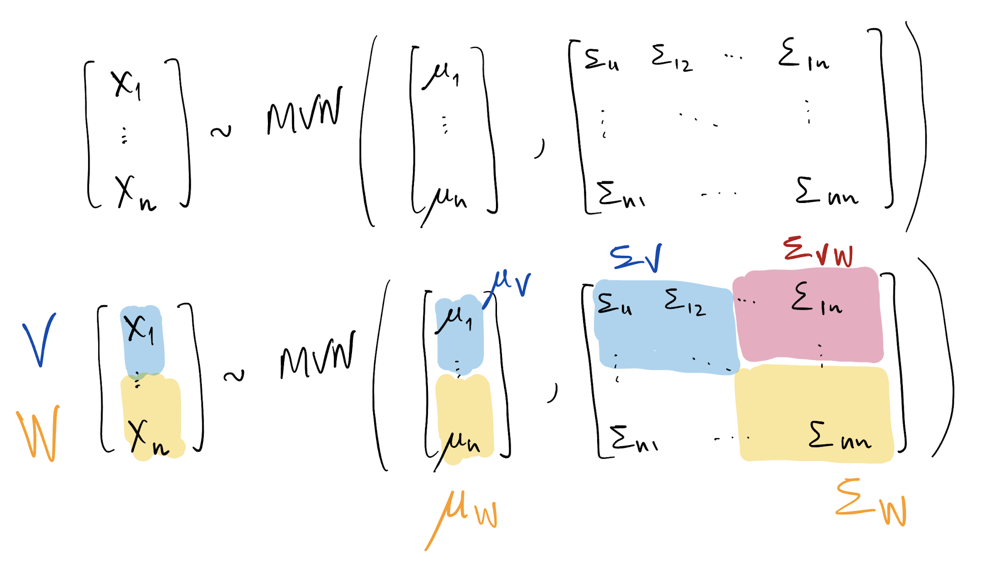
- Suppose X \sim MVN(x; \mu, \Sigma), where X is a column vector of dimension n\times 1
- \mu also has dimension n\times 1 whereas \Sigma is an n\times n symmetric and positive definite matrix
- E(X) = \mu and Var(X) = \Sigma
- Taking the subvector V = [X_1, \dots, X_k]^T, we have V \sim MVN(v; \mu_V, \Sigma_V) = MVN(v; \mu_{[1:k]}, \Sigma_{[1:k, 1:k]})
- Taking the subvector W = [X_{k+1}, \dots, X_n]^T, we have W \sim MVN(w; \mu_W, \Sigma_W) = MVN(w; \mu_{[k+1:n]}, \Sigma_{[k+1:n, k+1:n]})
- We also have Cov(V, W) = \Sigma_{VW} = \Sigma_{[1:k, k+1:n]} = \Sigma_{WV}^T = \Sigma_{[k+1:n, 1:k]}^T
Multivariate Normal
- Conditioning on jointly normal random vectors
- We have V | W=w \sim MVN(v; \mu_{V|W}, \Sigma_{V|W}), where \mu_{V|W} = \mu_V + \Sigma_{VW} \Sigma_W^{-1} (w - \mu_W) \Sigma_{V|W} = \Sigma_V - \Sigma_{VW} \Sigma_W^{-1} \Sigma_{VW}^T
- In particular, if \mu = 0 then \mu_{V|W} = \Sigma_{VW} \Sigma_W^{-1} w
- This is very important!
Multivariate Normal: density evaluation via Cholesky decompositions
Density of X \sim MVN(\mu, \Sigma) where X \in \Re^n is
p(x; \mu, \Sigma) = |2\pi \Sigma |^{-\frac{1}{2}} \exp\left\{ -\frac{1}{2}(x - \mu)^T \Sigma^{-1} (x - \mu) \right\}
|2\pi \Sigma |^{-\frac{1}{2}} = (2\pi)^{-\frac{n}{2}} | \Sigma |^{-\frac{1}{2}}, |\Sigma|^{-1} = \frac{1}{|\Sigma|}, and |\Sigma| = det\{\Sigma\}
Cholesky decomposition of \Sigma: it is the lower triangular matrix L such that L L^T = \Sigma
\Sigma^{-1} = L^{-T} L^{-1} where L^{-T} = (L^{-1})^T
\log \det(\Sigma) = 2 \sum_{i=1}^n \log L_{ii}
Therefore, if we have \Sigma, compute L then use it to evaluate density
Log-density most typically used in practice. This is then
\log p(x; \mu, \Sigma) = -\frac{n}{2} \log(2\pi) - \sum_{i=1}^n\log(L_{ii}) - \frac{1}{2}(x-\mu)^T L^{-T} L^{-1} (x-\mu)
Stochastic process modeling
- Goal is do model \{ Y(s), s \in D \}, an uncountable collection of random variables over D
- We want to be able to describe any collection of random variables!
- This is generally difficult
- Easier: make distributional assumptions for any finite collection of random variables
- In other words, define p(Y(s_1), \dots, Y(s_n)) for any possible finite set \cal L = \{ s_1, \dots, s_n \}
- Kolmogorov’s consistency conditions guarantee the existence of a stochastic process \{ Y(s), s \in D \} based on our definition of p(Y(s_1), \dots, Y(s_n))
Make your own stochastic process
- Define p(Y(s_1), \dots, Y(s_n)) for any possible finite set \cal L = \{ s_1, \dots, s_n \}
- Verify that Kolmogorov’s conditions are satisfied
Example: Poisson process
- On a continuous time domain D = \{t \in \Re: t \ge 0\}
- N(t) is an integer number of events of interest between times 0 and t, (1) N(t)\ge 0 and if s < t, then N(s) \le N(t) and N(t) - N(s) is the number of events occurred in (s, t]
- N(t) \sim Poisson(\lambda t) for some \lambda > 0
- \{ N(t), t \in D \} is called a Poisson process with rate \lambda
Example: Markov chains
- Take D = \{..., -2, -1, 0, 1, 2, \dots \}
- Consider an uncountable set of random variables \{ X(t), t \in D \}
- \{ X(t), t \in D \} is a Markov chain if
P( X(t+1) = j | X(t) = i_t, X(t-1) = i_{t-1}, \dots, X(0) = i_0 ) = P( X(t+1) = j | X(t) = i_t )
- Notice above: we are defining a finite dimensional joint distribution by listing all the conditionals!
\begin{align*}
P( X(t+1) = j,\ &X(t) = i_t,\ X(t-1) = i_{t-1},\ \dots,\ X(0) = i_0 ) =\\
& P(X(0) = i_0) \cdot P(X(1) = i_1 | X(0) = i_0) \cdots \\
& \cdots P( X(t+1) = j | X(t) = i_t,\ X(t-1) = i_{t-1},\ \dots,\ X(0) = i_0 )
\end{align*}
Markov chains: things to keep in mind
- We do not need in-depth knowledge of Markov chains
- We will use Markov-chain Monte Carlo (MCMC), which is based on the theory of discrete-time, continuous space Markov chains
- For a discrete-space Markov chain, and under some conditions, and with transition matrix P, at time t denoted with P^{(t)} = P \cdots [t times] \cdots P, we have \lim_{t \to \infty} P^{(t)}_{ij} = \pi_j
- \pi is called the stationary distribution
- General idea of MCMC: design and build a Markov chain whose stationary distribution is a target density \pi(\cdot); then, by running the Markov chain many times we will eventually get correlated samples of \pi(\cdot)
Gibbs sampling
- Suppose we want to extract samples from the joint distribution p(A, B)
- We know how to extract samples from p(A | B) and p(B | A)
- We then build a Markov chain \Theta_{t} = (A_t, B_t) on discrete time
- Fix some initial value \Theta_0 by setting A_0 = a, B_0 = b
- At time t we sample a new \Theta_{t} by updating its components: A_t \sim p(A | B = b_{t-1}) \qquad B_t \sim p(B | A = a_t)
- The stationary distribution for this Markov chain is p(A, B)
- In other words, we are alternating sampling from each conditional distribution to obtain (with large t) a (correlated) sample from the joint distribution
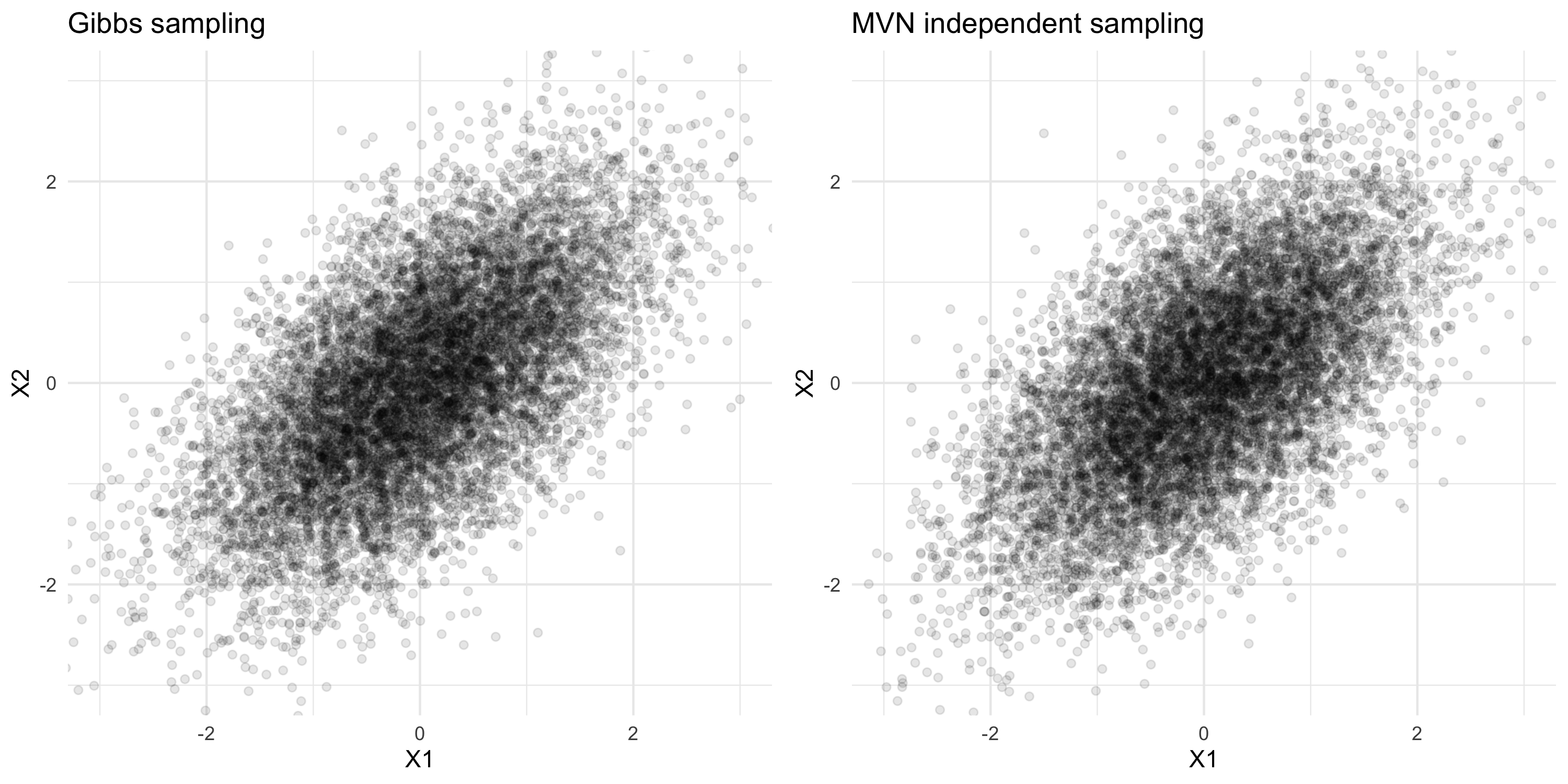
Gibbs sampling: toy example
- Suppose we want to extract samples from the joint distribution N\left(\begin{bmatrix} x_1 \\ x_2\end{bmatrix}; \begin{bmatrix} 0 \\ 0\end{bmatrix}, \begin{bmatrix}1 & \rho \\ \rho & 1 \end{bmatrix}\right)
- We know how to extract samples from p(X_1 | X_2=x_2) and p(X_2 | X_1=x_1):
\begin{align*}
p(X_1 | X_2=x_2) &= N(x_1; \rho x_2, 1-\rho^2) \\
p(X_2 | X_1=x_1) &= N(x_2; \rho x_1, 1-\rho^2)
\end{align*}
Gibbs sampling: toy example
![]()