Analysis of areal datasets

Introduction to areal data analysis

We have spent the last few lectures on point-referenced data
A major interest with point-referenced data is prediction at any spatial location
Spatial coordinates are non-random but live on the real line
In other words there is an infinite number of locations which we could predict
Contrast this to areal datasets: the number of “locations” or spatial units is finite and known beforehand
Example: U.S. states or counties

Introduction to areal data analysis

Domain is divided into non-intersecting regions
Each region has a set of neighbors, i.e. regions that share a border
Can build proximity matrix $W$ with elements $(w_{ij})_{i,j=1,n}$
We let $w_{ii} = 0$
$w_{ij}$ may reflect distance between area centroids
$w_{ij}$ may be set as 1 if $i$ and $j$ share a border
$w_{ij}$ can be seen as a weight, and we can let $\sum_j w_{ij} = 1$

Moran’s I

Statistic used to measure the strength of spatial association
Empirical estimate of the correlation function

$I = \frac{n \sum_i \sum_j w_{ij} (Y_i - \bar{Y})(Y_j - \bar{Y})}{(\sum_{i\neq j} w_{ij}) \sum_i (Y_i - \bar{Y})^2}$

$I$ is not strictly within $[-1, 1]$
Under null hypothesis of i.i.d. data, $I$ is asymptotically normal with mean $-1/(n-1)$

Moran’s I

Back to heart disease data

nb <- poly2nb(df_local, queen=TRUE)
lw <- nb2listw(nb, style="W", zero.policy=TRUE)
I <- moran(df_local$Data_Value, lw, length(nb), Szero(lw))[1]

moran.test(df_local$Data_Value, lw, alternative="two.sided")


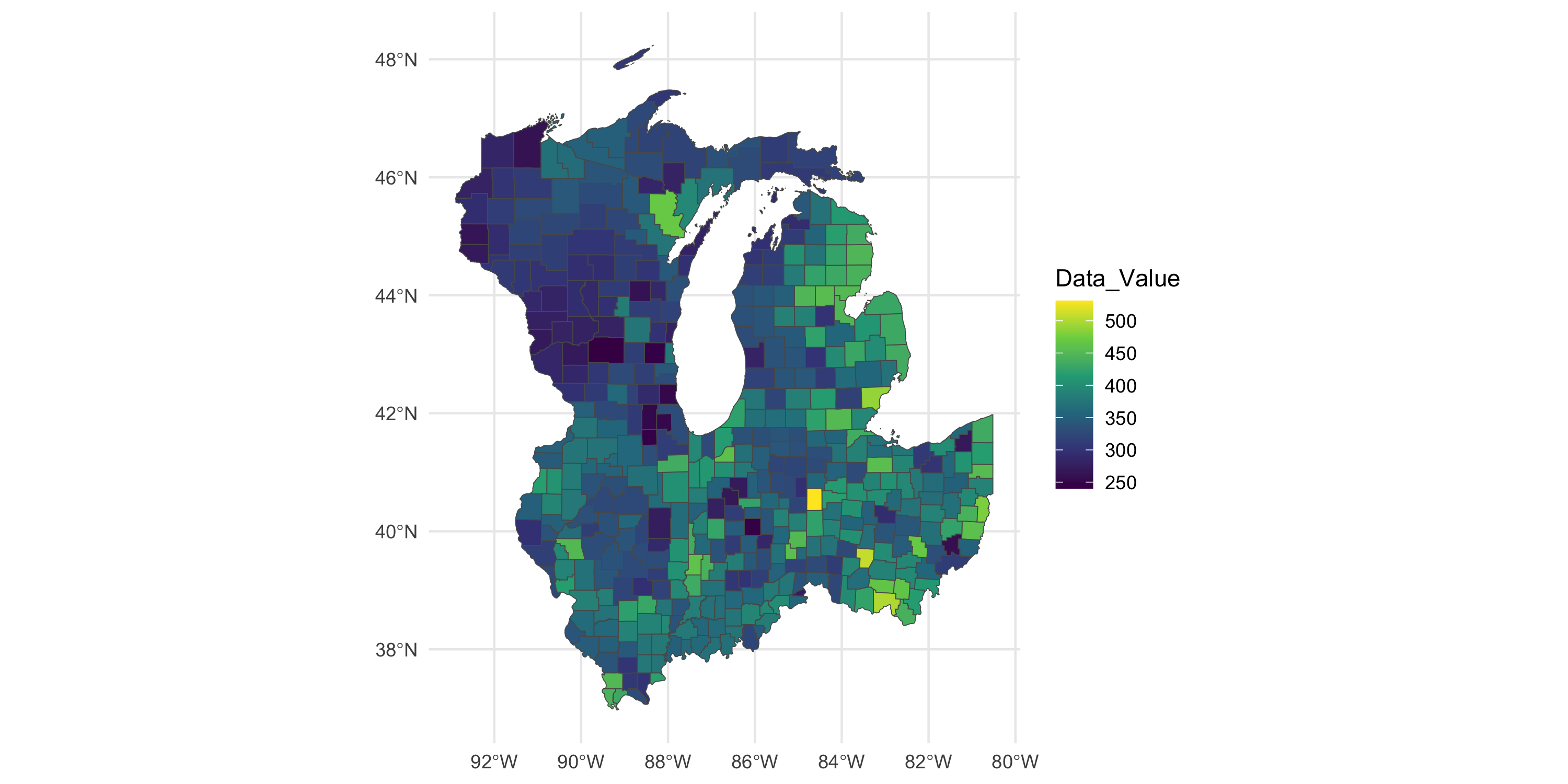
    Moran I test under randomisation

data:  df_local$Data_Value  
weights: lw    

Moran I statistic standard deviate = 15.968, p-value < 2.2e-16
alternative hypothesis: two.sided
sample estimates:
Moran I statistic       Expectation          Variance 
     0.4687127949     -0.0022935780      0.0008700179

Conditionally Autoregressive (CAR) models

Let $Y_i$ be our data at areal unit $i$
We assume $Y_i | Y_j, j\neq i \sim N\left(\sum_{j}b_{ij} y_{j}, \tau^2_i \right)\quad i=1,\dots,n$
We apply Brook’s lemma (see book p. 78) to find the joint density from all the full conditionals
We obtain

$Y \sim N(0, (I-B)^{-1}D )$

$B$ is the matrix of $b_{ij}$ and $D$ is diagonal with elements $d_{ii}=\tau^2_i$

Conditionally Autoregressive (CAR) models

Typical setup in practice:

$Y_i | Y_j, j\neq i \sim N\left(\frac{\rho \sum_{j}b_{ij} y_{j}}{\sum_{j}b_{ij}}, \frac{\sigma^2}{\sum_{j}b_{ij}} \right)\quad i=1,\dots,n$

This leads to joint density $Y \sim N(0, (1/\sigma^2)(D-\rho B)^{-1})$
In this case $D$ is diagonal with $i$ th element $d_{ii} = \sum_j b_{ij}$
Common and simple assumption is to let $b_{ij}=1$ if $i$ and $j$ share a border
Setting $\rho=1$ leads to an improper distribution: not a valid model for the data
An improper distribution can be used as a prior for random effects
$\rho<1$ leads to a proper distribution

Use of CAR model in Bayesian hierarchical model

As with point-referenced data, we can let

$\begin{align*} w &\sim CAR(B, D)\\ Y &= X\beta + w + \varepsilon,\ \varepsilon \sim N(0,\tau^2) \end{align*}$

Ideas for running MCMC?

The CAR-Leroux model

Used to model varying strengths of spatial association

$Y_i | Y_j, j\neq i \sim N\left(\frac{\rho \sum_{j}b_{ij} y_{j}}{\rho \sum_{j}b_{ij} + 1 - \rho }, \frac{\sigma^2}{\rho \sum_{j}b_{ij} + 1 - \rho } \right)\quad i=1,\dots,n$

ICAR model

Let the joint density for latent effects $w$ be

$w \sim N(0, \sigma^2 (D-B)^{-1} )$

$B$ is the adjacency or proximity matrix where $b_{ij} = 1$ if regions $i$ and $j$ share a border
$D$ is thus the diagonal matrix whose $i$ th diagonal element is $d_{ii} =$ the number of neighbors of region $i$
The proper CAR specification here would have covariance $(\tau(D-\rho B))^{-1}$ with $\rho<1$ . ICAR is obtained by letting $\rho=1$
The resulting ICAR model is improper and cannot be used to fit a dataset directly
Why improper? $D-B$ is singular and thus the resulting Gaussian density does not have a well-defined covariance matrix
However, it can be used as a prior for latent effects (which is what we are doing!)

ICAR model

The assumptions we have made on the joint density are a result of the following set of assumptions on the full conditional densities for $w_i$

$w_i | w_{-i} \sim N\left( \frac{\sum_{j: j\sim i} w_{ij}}{d_{ii}}, \frac{\sigma^2}{d_{ii}} \right)$

Here, the sum $\sum_{j: j\sim i}$ means we are summing over all the neighbors of $i$ . Notice $\sum_{j: j\sim i} w_{ij} = \sum_j b_{ij} w_{ij}$ using our definition of $B$

ICAR model

A property of this model is that we can write the joint density as a function of all pairwise differences

$p(w | \sigma^2) \propto \sigma^{n-\text{NC}} \exp \{ -\frac{1}{2\sigma^2} \sum_{i \sim j} (w_i - w_j)^2 \}$

Here, NC $=1$ if every region can be reached from any other region by traversing a sequence of neighbors
We also force the constraint $\sum_i w_i = 0$ .
Without this constraint, $w$ is not identifiable: suppose $c$ is a constant, then

$\sigma^{n-\text{NC}} \exp \{ -\frac{1}{2\sigma^2} \sum_{i \sim j} (w_i - w_j)^2 \} = \sigma^{n-\text{NC}} \exp \{ -\frac{1}{2\sigma^2} \sum_{i \sim j} ((w_i+c) - (w_j+c))^2 \}$

In the above example we cannot identify or distinguish $w$ from $w+c$ as both lead to the same (unnormalized) density value

Fitting a CAR model using `geostan`

$Y_i | Y_j, j\neq i \sim N\left(\mu + \frac{\rho \sum_{j}b_{ij} y_{j}}{\sum_{j}b_{ij}}, \frac{\sigma^2}{\sum_{j}b_{ij}} \right)\quad i=1,\dots,n$

Recall that our dataset df_local stores the overall rate of Heart disease

Fitting a CAR model using `geostan`

First, we need to create the proximity matrix
Use option style="B" for creating a binary matrix $B$ as defined earlier

C <- shape2mat(df_local, style = "B")
cp <- prep_car_data(C)

Range of permissible rho values:  -1.462401 1

Fitting a CAR model using `geostan`

Running MCMC is very simple
Stan typically rans an adaptive version of a Hamiltonian Monte Carlo algorithm
Here, we also specify family = auto_gaussian() to set the outcome distribution as Gaussian
Note that Stan can fit HMC to non-Gaussian models
Option to fit more than 1 chain to check convergence

fit <- stan_car(Data_Value ~ 1,
                car_parts = cp,
                data = df_local,
                family = auto_gaussian(),
                iter = 5000, chains = 1)

  location scale
1      356   204
  df location scale
1 10        0   102
  lower upper
1  -1.5     1

SAMPLING FOR MODEL 'foundation' NOW (CHAIN 1).
Chain 1: 
Chain 1: Gradient evaluation took 0.000602 seconds
Chain 1: 1000 transitions using 10 leapfrog steps per transition would take 6.02 seconds.
Chain 1: Adjust your expectations accordingly!
Chain 1: 
Chain 1: 
Chain 1: Iteration:    1 / 5000 [  0%]  (Warmup)
Chain 1: Iteration:  500 / 5000 [ 10%]  (Warmup)
Chain 1: Iteration: 1000 / 5000 [ 20%]  (Warmup)
Chain 1: Iteration: 1500 / 5000 [ 30%]  (Warmup)
Chain 1: Iteration: 2000 / 5000 [ 40%]  (Warmup)
Chain 1: Iteration: 2500 / 5000 [ 50%]  (Warmup)
Chain 1: Iteration: 2501 / 5000 [ 50%]  (Sampling)
Chain 1: Iteration: 3000 / 5000 [ 60%]  (Sampling)
Chain 1: Iteration: 3500 / 5000 [ 70%]  (Sampling)
Chain 1: Iteration: 4000 / 5000 [ 80%]  (Sampling)
Chain 1: Iteration: 4500 / 5000 [ 90%]  (Sampling)
Chain 1: Iteration: 5000 / 5000 [100%]  (Sampling)
Chain 1: 
Chain 1:  Elapsed Time: 1.267 seconds (Warm-up)
Chain 1:                0.547 seconds (Sampling)
Chain 1:                1.814 seconds (Total)
Chain 1:

Fitting a CAR model using `geostan`

Checking MCMC output proceeds as usual
In this case we need to extract information from the fit object

ext_mcmc <- extract(fit$stanfit)

Fitting a CAR model using `geostan`

The package also provides useful functions for diagnostics

Fitting a CAR model using `geostan`

We can check whether there is spatial dependence in the residuals by computing Moran’s I on them

model_residuals <- residuals(fit)$mean

df_local <- df_local %>% mutate(car_resid = model_residuals)
car_resid_plot <- ggplot(data=df_local) +
  geom_sf(aes(fill=car_resid)) +
  theme_minimal() +
  scale_fill_viridis_c() 

moran.test(model_residuals, lw, alternative="two.sided")


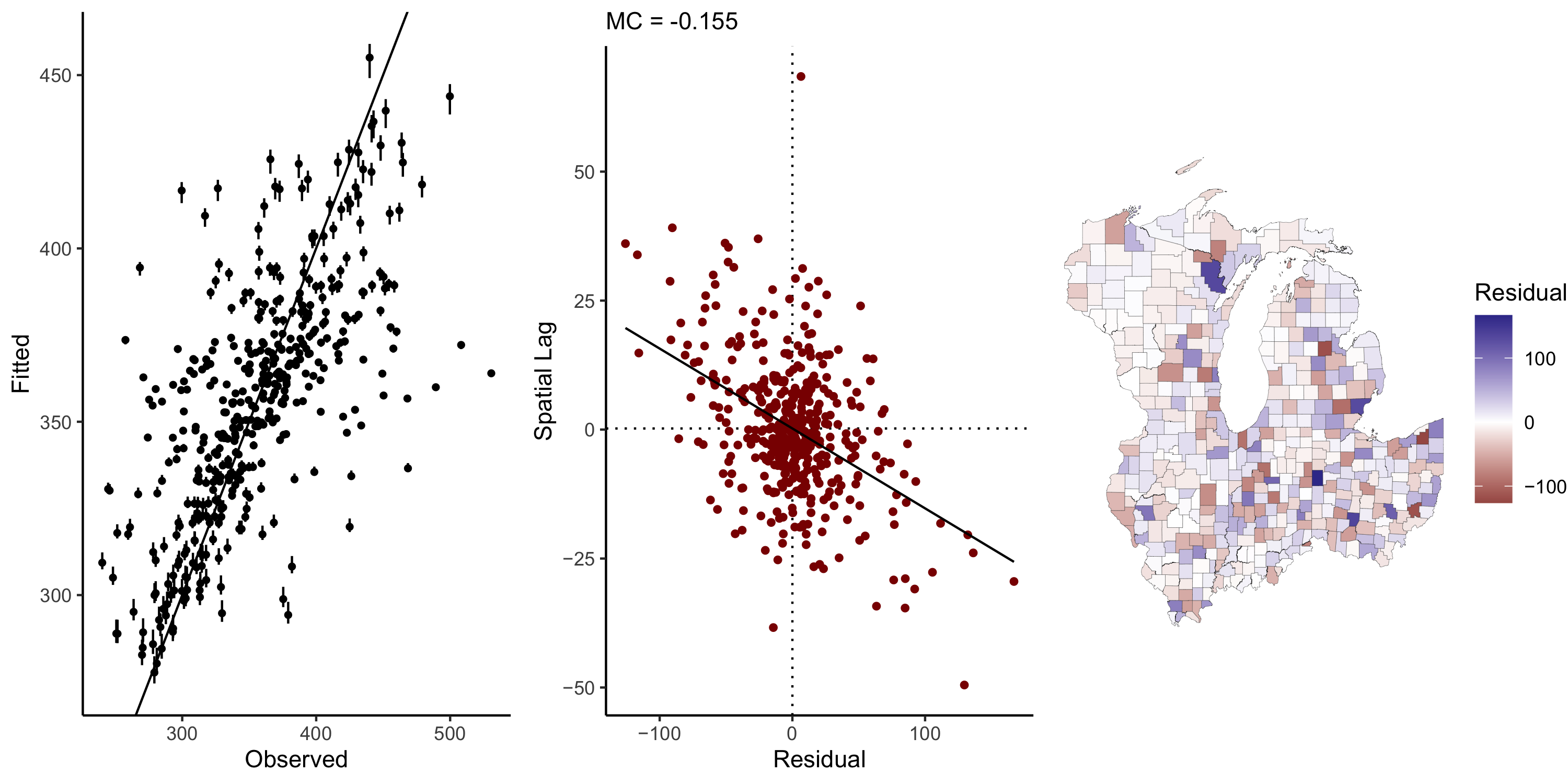
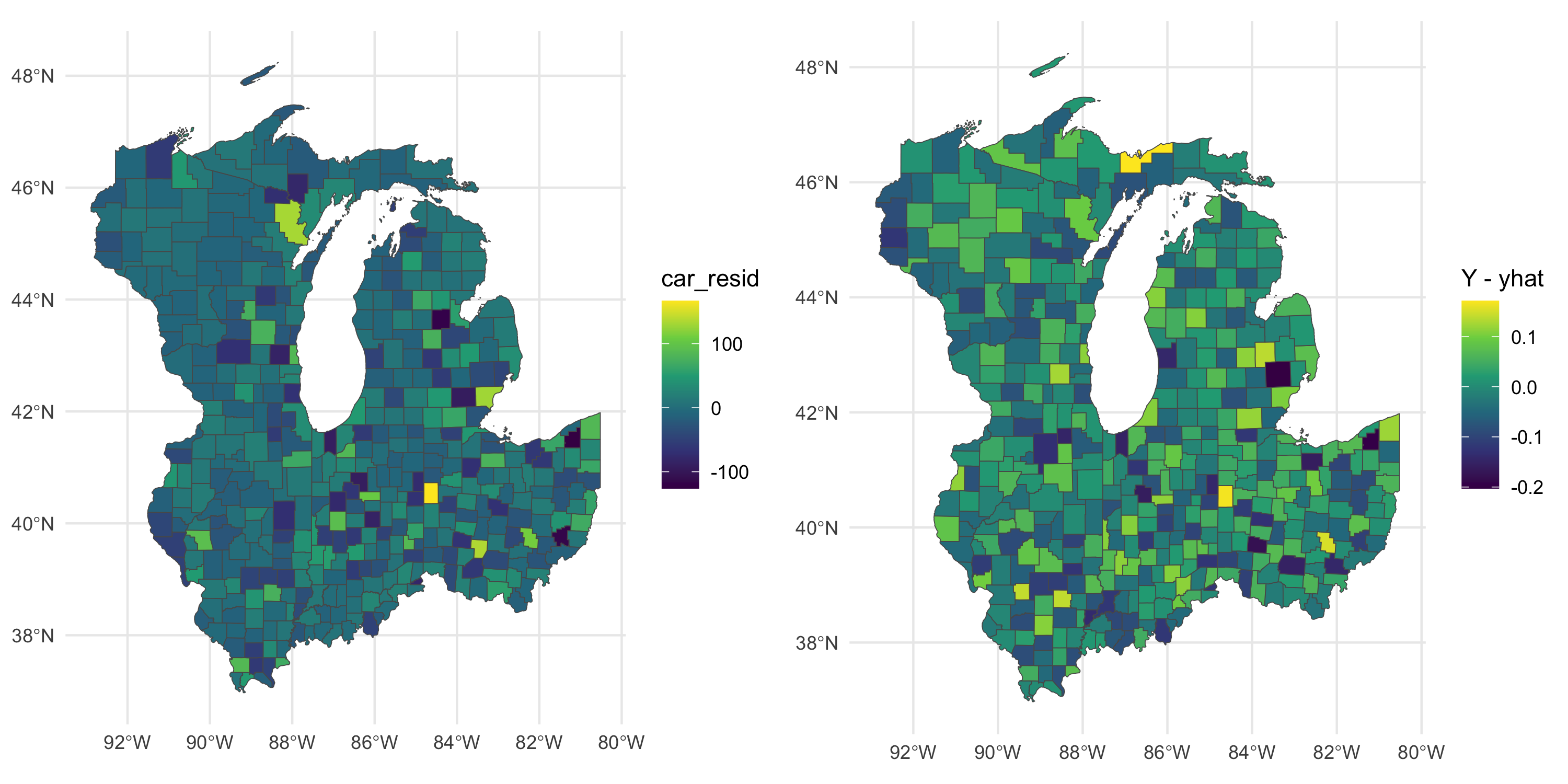
    Moran I test under randomisation

data:  model_residuals  
weights: lw    

Moran I statistic standard deviate = -5.1855, p-value = 2.154e-07
alternative hypothesis: two.sided
sample estimates:
Moran I statistic       Expectation          Variance 
    -0.1548429467     -0.0022935780      0.0008654362

In this case there is still spatial dependence in the residuals
We did not use any covariates
One worry we should have: do we need an offset?
Offset: an additive or multiplicative constant that adjusts the observed value by the size of the relative area
For example, if we were counting the absolute number of cases, we should offset by population
Not doing so may result in a residual pattern that looks just like the area size!
In the heart disease case we have data per 100k population so we do not need offsets

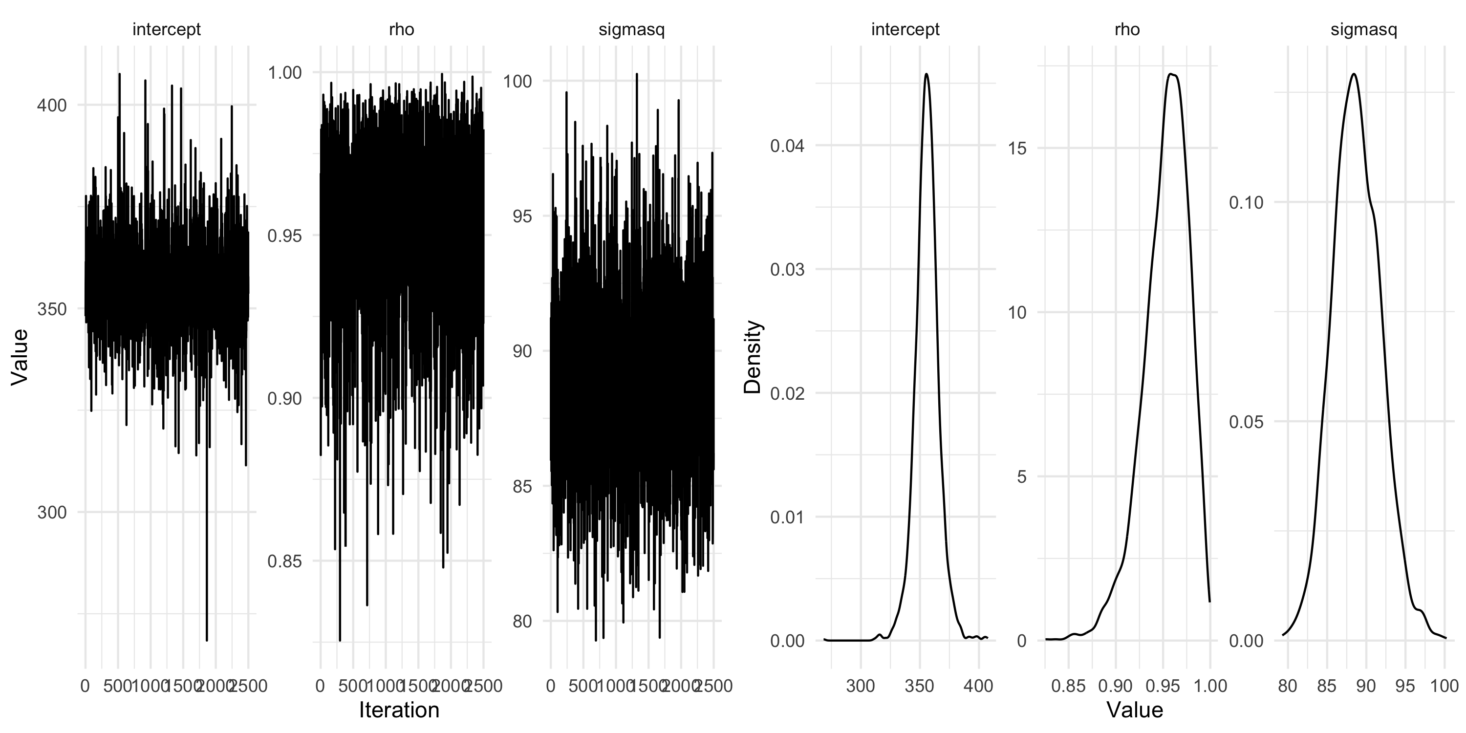
Fitting a CAR model using `geostan`

The model we saw did not allow for the introduction of measurement error
We thus fit a CAR model to the data directly
geostan seems to lack the ability to fit a latent model to Gaussian data

Simultaneously Autoregressive models (SAR)

In this case we model all outcomes $Y$ as arising from independent innovations:
Define $B$ as earlier as a weight matrix, possibly binary
Define $R$ as diagonal with region-specific diagonal entries $r_{ii}$
We can simplify and let $R = \sigma^2 I_n$

$\begin{align*} \varepsilon &\sim N(0, R)\\ Y &= X\beta + (I_n - \rho B)^{-1} \varepsilon \end{align*}$

As a result of this assumption, we have

$Y \sim N(X\beta, (I_n - \rho W)^{-1} R (I_n - \rho W)^{-T})$

This implies that the precision matrix is found as $(I_n - \rho W)^T R^{-1} (I_n - \rho W)$
Any SAR model can be cast as a CAR model, the converse is not true
CAR models are thus a larger class

Crazy idea: fit a GP to areal data using centroids?

Gaussian “Process” is a misnomer for the model we are fitting
We do not want to estimate a smooth infinite-dimensional surface on a spatial domain
CAR/SAR models take into account neighbor structure
They do so for ease of computations and interpretation
Restrictions can be hard to swallow

Gaussian “Processes” in areal data?

All we need is a coordinate system for the areal dataset
First option is to use regions’ centroids
Distance between centroids is the average distance between pairs of points across regions
Alternatives: compute centroids using population distribution within each region
Once we have centroids, we can compute distances!
Once we can compute distances, we can model covariance
The covariance function will lead to a fixed set of pairwise correlations between regions
Because we are not interested in predictions at new locations, we technically do not even need a covariance function!

Gaussian “Processes” in areal data?

For the vector $Y$ of outcomes at each region, we have

$\begin{align*} w | \theta &\sim N(0, C_{\theta})\\ Y | \beta, \tau^2, w &\sim N(X\beta + w, \tau^2 I_n) \end{align*}$

Here, $C_{\theta}(i, j)$ will be interpreted as the “strength of connection” between $i$ and $j$
The corresponding graphical model interpretation is obtained by looking at $C_{\theta}^{-1}(i,j)$

Experiment

Prepare the coordinate matrix and the data (centered, for simplicity)

coords <- df_local %>% st_drop_geometry() %>% dplyr::select(X_lon, Y_lat) %>% as.matrix()
colnames(coords) <- c("Var1", "Var2")
Y <- df_local$Data_Value - mean(df_local$Data_Value)
X <- rnorm(length(Y)) %>% matrix(ncol=1)

Experiment

Fit a GP using any package
In this case, meshed provides adaptive MCMC for covariance hyperparameters, which is useful

set.seed(1)
fit_meshed <- meshed::spmeshed(Y, X, coords, n_samples=500, n_burnin=500, n_thin=2, prior=list(phi=c(0.1,20)),
                         settings=list(forced_grid=FALSE, cache=FALSE),
                         debug=list(sample_beta=FALSE), verbose=3)

Bayesian Meshed GP regression model fit via Markov chain Monte Carlo
Sending to MCMC.
33.5% elapsed:   978ms (+  879ms). ETR: 2.14s. 
  theta: Metrop. acceptance 24.50%, average 25.90% 
  theta = 1.640 4.592 
  tausq = (1) 0.208762 
  lambda = 55.684 

66.9% elapsed:  1863ms (+  884ms). ETR: 1.02s. 
  theta: Metrop. acceptance 22.50%, average 26.02% 
  theta = 1.548 3.884 
  tausq = (1) 0.399729 
  lambda = 51.697 

MCMC done [2.647s]

Experiment

meshed returns a data frame which needs to be used because coordinates may be in a different order compared to input coordinates

meshed_fitted <- fit_meshed$yhat_mcmc %>% meshed::summary_list_mean()
meshed_out <- fit_meshed$coordsdata %>% 
  mutate(yhat=meshed_fitted) %>% 
  dplyr::select(-forced_grid) %>%
  rename(X_lon = Var1, Y_lat=Var2)

Join with original data and run Moran’s test

df_local_meshed <- df_local %>% mutate(Y=Y)
df_local_meshed <- df_local_meshed %>% left_join(meshed_out)

df_local_meshed %>% with(moran.test(Y-yhat, lw, alternative="two.sided"))


    Moran I test under randomisation

data:  Y - yhat  
weights: lw    

Moran I statistic standard deviate = -3.4487, p-value = 0.0005634
alternative hypothesis: two.sided
sample estimates:
Moran I statistic       Expectation          Variance 
    -0.1040171021     -0.0022935780      0.0008700435

Experiment

Map of the residuals

meshed_resid_plot <- ggplot(data=df_local_meshed) +
  geom_sf(aes(fill=Y-yhat)) +
  theme_minimal() +
  scale_fill_viridis_c()

Experiment

Compare with CAR

grid.arrange(car_resid_plot, meshed_resid_plot, nrow=1)

Areal data as aggregates of point patterns

Recall what point-pattern data are
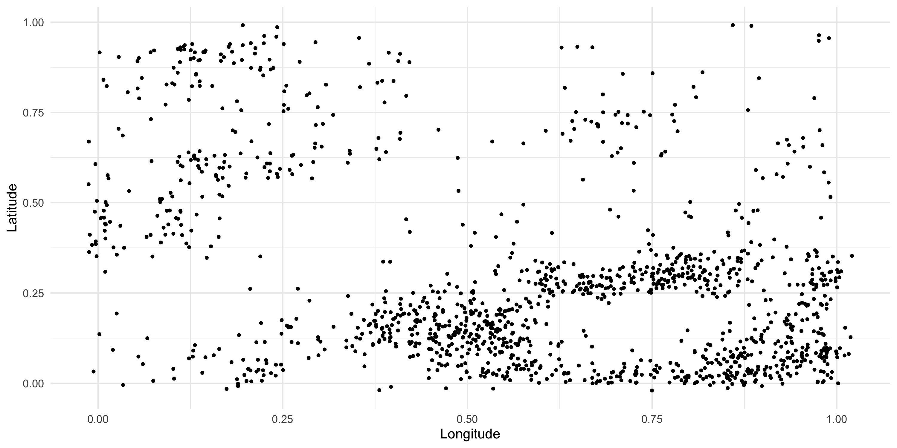
We have spatial information about the spatial occurence of some event
We are mostly interested with learning about the pattern of locations
Where did the events occur?
The dataset this gives rise to is a pattern of locations (points)
Our dataset boils down to the set of observed locations $\{ S_1, \dots, S_n \}$
We model these locations as random
If we were also interested on other information about the events we would talk of a marked point pattern. In that case both $\{ S_1, \dots, S_n \}$ and $\{Y(S_1), \dots, Y(S_n)\}$ are random
Recall with point-referenced data we only model $\{Y(s_1), \dots, Y(s_n)\}$ assuming the locations are not random (i.e. known, fixed, constant)

Areal data as aggregates of point patterns

Suppose we want to model the spread of a disease
Or the spread of a type of invasive species
Or the occurrence of forest fires
Or the location of traffic accidents

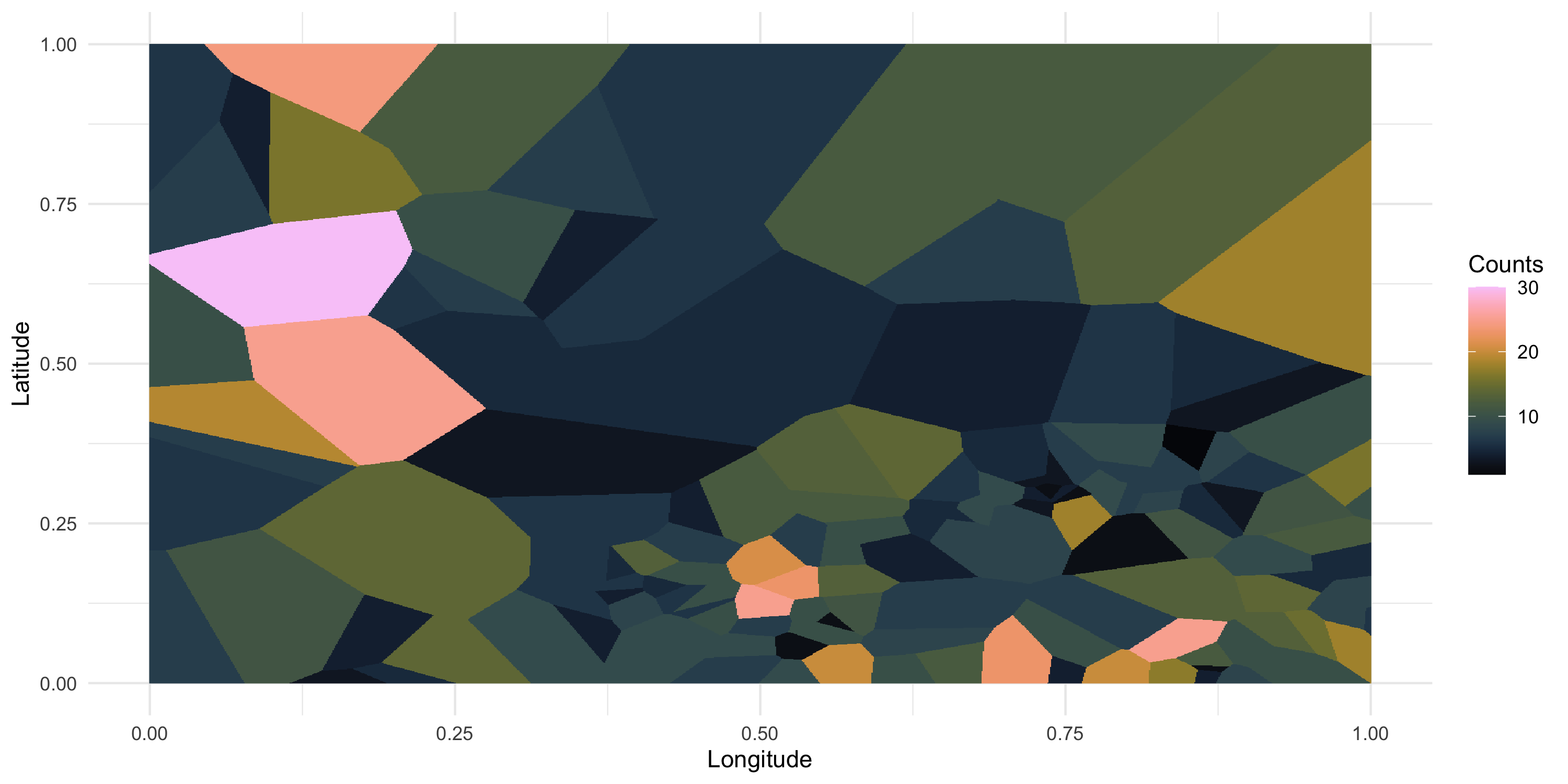
Areal data as aggregates of point patterns

Aggregation into areas

Rather than directly using the dataset of locations, we summarize information across pre-specified areas
Typically, we count how many events occurred in each area

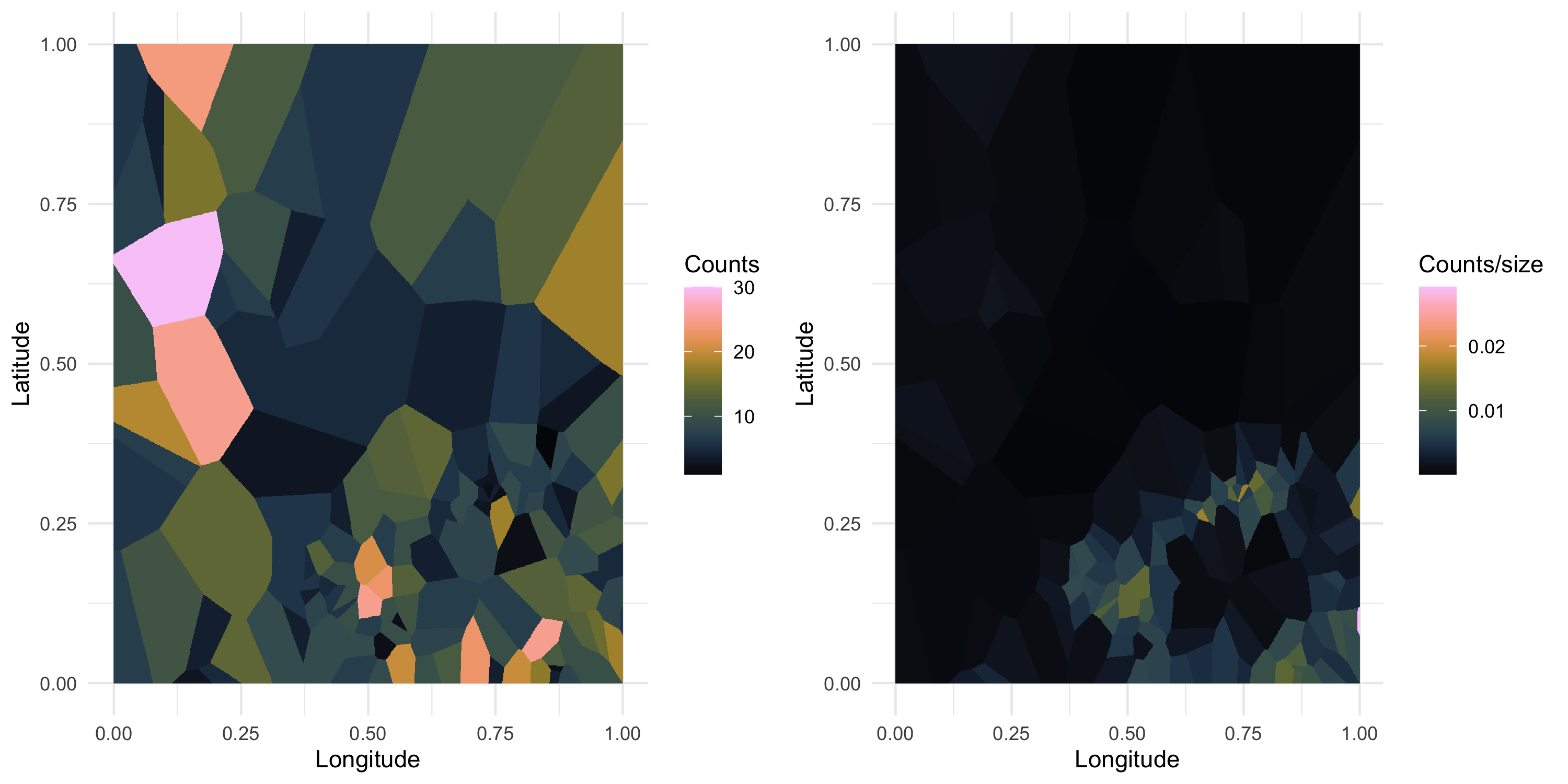
Areal data as aggregates of point patterns

Be mindful of the size of the areas when we count!

Areal data as aggregates of point patterns

Motivation/Scenario 1
- In many cases, we only have information at an aggregate level
- Even if we have exact location of “disease” we may only have socio-demographic info at zip-county-state level
- See book Section 6.4
Motivation/Scenario 2
- We are interested in the intensity of the underlying process
- Higher intensity means larger rate of occurrence of events
- Estimating intensity continuously is a difficult problem in 2+ dimensions
- By aggregating, we can simplify (i.e. approximate) and make the problem manageable
- See book Section 8 (specifically 8.4.3)

Areal data as aggregates of point patterns

Let’s get modeling!

We have a set of areas or spatial indices or centroids or coordinates $\{s_1, \dots, s_n\}$
We have counts at those locations: $\{ Y_1, \dots, Y_n \}$ where $Y_i=Y(s_i)$
Model those counts as Poisson random variables
Set up a spatial GLM model with log link
Call $E_i$ the size of area $i$ . This is problem dependent!
Example: if $Y_i$ are disease counts, $E_i$ should be the expected number of counts
Call $n_i$ the population size at $i$ (not a random variable), then $E_i = n_i \cdot \bar{r}$ where $\bar{r}$ is the overall occurrence rate across the region

$\begin{align*} Y_i &\sim Poisson(E_i \eta_i) \end{align*}$

Our goal is to estimate $\eta_i$ , i.e. the relative intensity or risk at area $i$

Conjugate Bayesian model for Poisson counts

$\begin{align*} \eta_i &\sim Gamma(a, b)\\ Y_i|\eta_i &\sim Poisson(E_i \eta_i) \end{align*}$

The Gamma prior on $\eta_i$ is conjugate to the Poisson model for $Y_i$
This implies that the posterior is also a Gamma distribution
The posterior can be derived analytically and it is

$\begin{align*} p(\eta_i | Y) = p(\eta_i | Y_i) &= Gamma(y_i + a, E_i + b) \end{align*}$

Therefore the Bayesian point estimate for $\eta_i$ is $\hat{\eta}_i = E(\eta_i | Y) = \frac{y_i + a}{E_i + b}$
Conjugacy is convenient! However, it is difficult to model spatial dependence via a Gamma distribution

Spatial Bayesian model for Poisson counts: setup

$\begin{align*} \psi_i &= X_i^\top \beta + w_i + \varepsilon_i \\ Y_i|\eta_i &\sim Poisson(E_i e^\psi_i) \end{align*}$

$\psi_i = \log \eta_i$ is the log-relative risk or log-intensity
We now have $w_i$ and $\varepsilon_i$ which we can use to model
- spatial correlation
- non-spatial “noise” in the observed counts
What priors could we use for $w$ and $\varepsilon$ ?

Spatial Bayesian model for Poisson counts

$\begin{align*} \varepsilon_i &\sim N(0, \tau^2)\\ \theta &\sim p(\theta)\\ \{ w_i \}_{i=1}^n &\sim \text{Gaussian with sparse graph}(0, C_{\theta}) \\ \psi_i &= X_i^\top \beta + w_i + \varepsilon_i \\ Y_i|\eta_i &\sim Poisson(E_i e^\psi_i) \end{align*}$

Spatial Bayesian model for Poisson counts: example 1

$\begin{align*} \{ w_i \}_{i=1}^n &\sim ICAR \end{align*}$

We can use a CAR model based on neighbor relationships between areas

Spatial Bayesian model for Poisson counts: example 2

$\begin{align*} \{ w_i \}_{i=1}^n &\sim \text{DAG-Gaussian}(0, \tilde{C}_{\theta}) \end{align*}$

We can use a DAG-based model using centroids and a user-defined covariance function
Notice this is not technically a GP prior because we have areas
However, setting up this model proceeds the same way as for a DAG-GP case (see previous slides)

Spatial Bayesian model for Poisson counts: computations

$\begin{align*} \varepsilon_i &\sim N(0, \tau^2)\\ \theta &\sim p(\theta)\\ \{ w_i \}_{i=1}^n &\sim \text{Gaussian with sparse graph}(0, C_{\theta}) \\ \psi_i &= X_i^\top \beta + w_i + \varepsilon_i \\ Y_i|\eta_i &\sim Poisson(E_i e^\psi_i) \end{align*}$

Regardless of our prior choice for $w$ , MCMC generally works via Metropolis-within-Gibbs

Move $\tau^2$ with target $p(\tau^2 | Y, \dots)$
Move $\theta$ with target $p(\theta | Y, \dots)$
Move $\{w_i\}_{i=1}^n$ with target $p(w | Y, \dots)$
Move $\beta$ with target $p(\beta | Y, \dots)$

Here, we let “ $\dots$ ” refer to all other unknowns in the model

Spatial Bayesian model for Poisson counts: computations

Recall that when the model was Gaussian, i.e. $Y|\dots\sim N(\dots)$ and with conjugate priors, we had:

Gibbs sample $\tau^2$ with target $p(\tau^2 | Y, \dots)$ (Inverse Gamma)
Update $\theta$ with target $p(\theta | Y, \dots)$ (Metropolis step) Tuning/choice of update is important for efficiency!
Gibbs sample $\{w_i\}_{i=1}^n$ with target $p(w | Y, \dots)$ (Gaussian in 1 block or visiting each node of the graphical model)
Gibbs sample $\beta$ with target $p(\beta | Y, \dots)$ (Gaussian)

Thus, Metropolis-within-Gibbs but predominantly a Gibbs sampler with analytically tractable distributions. Now we have a Poisson outcome model.

Spatial Bayesian model for Poisson counts: computations

This model is not conjugate
Recall: if the full conditional posterior are available analytically then we can run a Gibbs sampler
In that case, we would have a conditionally conjugate model
The model above is not conditionally conjugate
Here, $p(w | Y, \theta, \beta, \tau^2)$ is not available analytically
The other full conditional densities are also typically not conditionally conjugate
$p(w | Y, \theta, \beta, \tau^2)$ is typically the highest-dimensional and hence most problematic

Spatial Bayesian model for Poisson counts: computations

With $Y|\dots\sim Poisson(\dots)$ we have:

Update $\tau^2$ with target $p(\tau^2 | Y, \dots)$ (Metropolis step) Tuning/choice of update is important for efficiency!
Update $\theta$ with target $p(\theta | Y, \dots)$ (Metropolis step) Tuning/choice of update is important for efficiency!
Update $\{w_i\}_{i=1}^n$ with target $p(w | Y, \dots)$ (Metropolis step) Tuning/choice of update is important for efficiency!
Update $\beta$ with target $p(\beta | Y, \dots)$ (Metropolis step) Tuning/choice of update is important for efficiency!

At each step we need to

Formulate a proposal distribution
Accept or reject the proposed value
Tune the proposal according to some criterion

Doing so for each step complicates matters significantly

Spatial Bayesian model for Poisson counts: computations

Difficult setup of MCMC or poor practical performance of MCMC in high-dimensional non-Gaussian settings lacking (conditional) conjugacy
Motivates development of MCMC-free posterior computing algorithms
See e.g. Laplace approximations, Integrated Nested Laplace Approximation (INLA), Variational approximations, Expectation propagation…
Also motivates research on new MCMC methods that are more efficient
Gradient-based MCMC: Metropolis-adjusted Langevin, Preconditioned Langevin, Hamiltonian Monte Carlo, No-U-Turn sampler, Riemannian-manifold MCMC…
Ease of adaptation is often an important part of algorithm choice

Review: Metropolis updates

Recall the general problem of Metropolis-based updates
We want to create a Markov chain $\{ X_m \}m\ge 0$ that will ultimately converge to a target density $p(x)$ of a random vector $X \in \Re^d$
To do so, we build a proposal distribution $q(\cdot | \cdot)$ that suggests the next value for $X$ in the chain
At step $m$ , we thus generate $X^*_{m+1} \sim q(\cdot | X_{m})$
We then accept or reject $X^*_{m+1}$ based on the Hastings ratio
If accepted, we move to $X^*_{m+1}$ , otherwise we do not move. In other words, accept means $X_{m+1} = X^*_{m+1}$ , reject means $X_{m+1} = X_{m}$
The question is how to choose $q(\cdot | \cdot)$ such that the resulting algorithm is efficient

Example: Random walk Metropolis

Fix $r$ , then let

$q(x | x_{\text{old}}) = N(x; x_{\text{old}}, r^2 I_d)$ In other terms, let $u \sim N(0, I_d)$ , we accept/reject the following proposal: $x_{\text{prop}} = x_{\text{old}} + r u$

We saw this is not very easy to tune and requires at least some adaptation for $r$

Example: Metropolis-adjusted Langevin algorithm (MALA)

Take the target density $p(x)$ and compute its gradient $\nabla p(x)$

Fix $\varepsilon$ , then let

$q(x | x_{\text{old}}) = N(x; x_{\text{old}} + \frac{\varepsilon^2}{2} \nabla p(x_{\text{old}}), \varepsilon^2 I_d)$ In other terms, let $u \sim N(0, I_d)$ , we accept/reject the following proposal: $x_{\text{prop}} = x_{\text{old}} + \frac{\varepsilon^2}{2} \nabla p(x_{\text{old}}) + \varepsilon u$ This proposal takes into account some local information about the distribution which we ultimately want to sample from

Example: MALA with preconditioner

Take the target density $p(x)$ and compute its gradient $\nabla p(x)$

Fix $\varepsilon$ and $M$ , then let

$q(x | x_{\text{old}}) = N(x; x_{\text{old}} + \frac{\varepsilon^2}{2} M \nabla p(x_{\text{old}}), \varepsilon^2 M)$ In other terms, let $u \sim N(0, I_d)$ , we accept/reject the following proposal: $x_{\text{prop}} = x_{\text{old}} + \frac{\varepsilon^2}{2} M \nabla p(x_{\text{old}}) + \varepsilon M^{\frac{1}{2}} u$

$M^{\frac{1}{2}}$ is a matrix square root (e.g. Cholesky)
This proposal takes into account some local information about the distribution which we ultimately want to sample from
We can use $M$ to further improve upon MALA but fixing it may be difficult. Alternatively:
- $M = ( - \nabla^2 p(x_{\text{old}}) )^{-1}$ (inverse of negative Hessian matrix of the target density) leads to the simplified Riemannian-manifold MALA (Girolami and Calderhead 2010)
- $M$ can be adapted using $( - \nabla^2 p(x) )^{-1}$ leading to a faster and more efficient algorithm in spatial models (P and Dunson 2024)
R package meshed uses MALA with adaptive preconditioner for non-Gaussian spatial models