Low-rank GPs and the Predictive GP

Introduction

We have introduced GP models
Spatial GP models are priors over 2D surfaces (or 2D functions)
Specifying the GP boils down to modeling covariance
GPs can be used as part of a Bayesian hierarchical model
We look for the posterior of a Bayesian model
When the joint posterior is “difficult” we design MCMC algorithms to sample from it
Models based on GPs scale poorly in terms of memory and flops and time

Scalable GP models

We will now consider building special GPs that can scale to larger datasets
There is no free lunch: scalability comes at a price
As usual, we will need to consider trade-offs and make decisions based on our modeling goals
Typically, we will restrict dependence across space, simplifying its structure
By restricting spatial dependence we will speed up computations
We will also lose in flexibility relative to an unrestricted GP

Graphical model interpretation of multivariate Gaussian random variables

Suppose we have a set of $n$ random variables $X_1, \dots, X_n$
Call $X = (X_1, \dots, X_n)^\top$
Assume that $X \sim N(0, \Sigma)$
$p(X_1, \dots, X_n) = p(X) = N(X; 0, \Sigma)$

Graphical model interpretation of multivariate Gaussian random variables

Using the properties of probability we can write $\begin{align*} p(X_1, \dots, X_n) &= p(X_1) p(X_2 | X_1) \cdots p(X_n | X_1, \dots, X_{n-1})\\ &= \prod_i^n p(X_i | X_{[1:i-1]}) \end{align*}$ where $X_{[1:i-1]} = (X_1, \dots, X_{i-1})^\top$
What is $p(X_i | X_{[1:i-1]})$ ?

Graphical model interpretation of multivariate Gaussian random variables

What is $p(X_i | X_{[i-1]})$ ?
$p(X_i | X_{[1:i-1]})$ is a conditional Gaussian distribution
This is the same distribution that we get when we predict $X_i$ using $X_{[1:i-1]}$ $N(X_i; H_i X_{[1:i-1]}, R_i)$ where $H_i = \Sigma(i, [1:i-1]) \Sigma([1:i-1], [1:i-1])^{-1}$ and $R_i = \Sigma(i, i) - H_i \Sigma([1:i-1], i)$ .

Graphical model interpretation of multivariate Gaussian random variables

Because $p(X_1, \dots, X_n) = \prod_i^n p(X_i | X_{[i]})$ , we can draw a DAG according to which the joint density factorizes
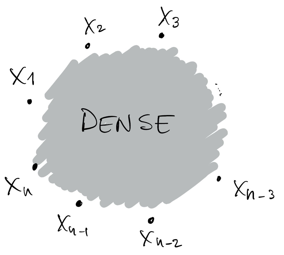
The number of edges cannot be any larger (for a DAG)
If we added even just a single directed edge, the graphical model would form a cycle
This DAG is dense
We can attribute the computational complexity of GPs to the fact that their DAGs are dense
Scaling GPs can be cast as a problem of sparsifying this DAG
In other words, methods to remove edges from the DAG in a smart way

Graphical model interpretation of multivariate Gaussian random variables

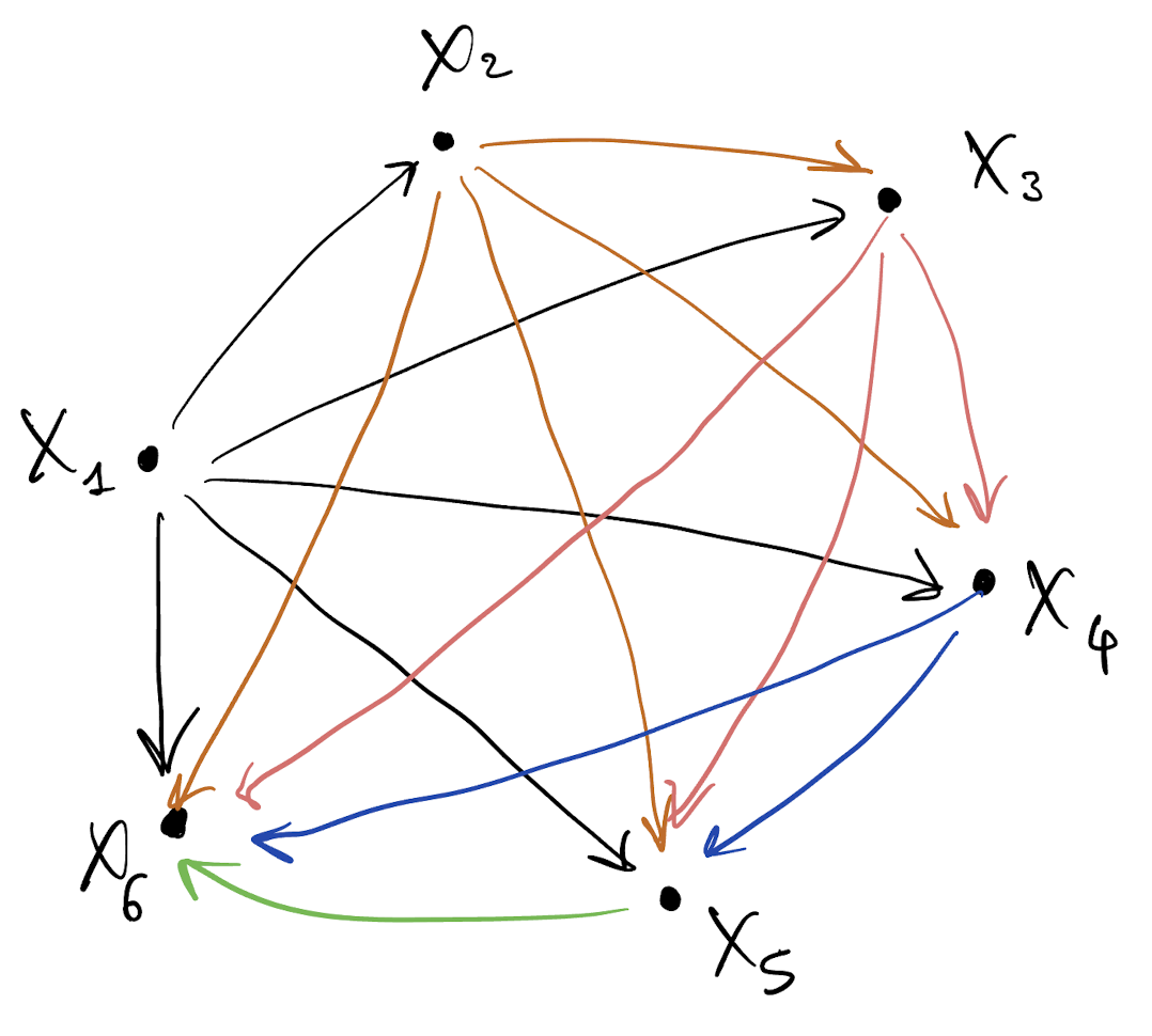
Draw a DAG for $p(X_1, \dots, X_6) = p(X_1) p(X_2 |$ ??? $) p(X_3 |$ ??? $) \cdots p(X_6 |$ ??? $)$

Graphical model interpretation of multivariate Gaussian random variables

Draw a DAG for $p(X_1, \dots, X_6)$
This DAG is dense

Graphical model interpretation of multivariate Gaussian random variables

Draw a DAG for $p(X_1, \dots, X_n)$
This DAG is dense

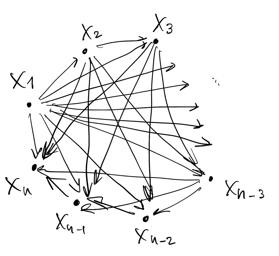
Graphical model interpretation of multivariate Gaussian random variables

Draw a DAG for $p(X_1, \dots, X_n)$
This DAG is dense

Low-rank Gaussian Processes

Dense dependence follows from assuming a GP
$X(\cdot) \sim GP$ implies $X_{\cal L} \sim N(0, \Sigma)$ implies dense DAG
We want $X(\cdot) \sim \text{???}$ leading to a simpler DAG that is sparse

Then, remember how we build a stochastic process:

Define the joint distribution for any finite set of random variables
Check Kolmogorov’s conditions
Result: there is a stochastic process whose finite dimensional distribution is the one we chose

Low-rank Gaussian Processes

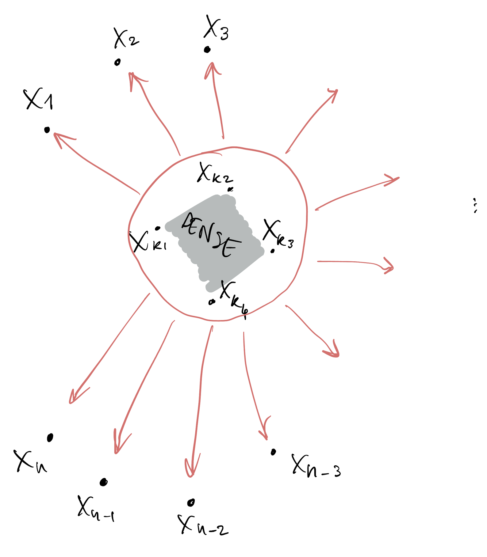
Assume dense dependence for only a small set of variables
All the others are assumed conditionally independent
We assume the resulting joint density factorizes according to this DAG (see prelim slides)

Low-rank Gaussian Processes

Suppose from $n$ variables we allow dense dependence for only $k$ of them
$p(X_1, \dots, X_n) = p(X_1, \dots, X_k, X_{k+1}, \dots, X_n)$
The finite dimensional distribution we assume has the form

$\begin{align*} p^*(X_1, \dots, X_n) &= p(X_1, \dots, X_k) \prod_{i=k+1}^n p(X_i | X_1, \dots, X_k) \end{align*}$

We then assume that all these densities are Gaussian

$\begin{align*} p^*(X_1, \dots, X_n) &= N(X_{[1:k]}; 0, \Sigma_{[1:k]}) \prod_{i=k+1}^n N(X_i; H_i X_{[1:k]}, R_i) \end{align*}$

where, as usual,

$\begin{align*} H_i &= \Sigma_{i, [1:k]} \Sigma_{[1:k]}^{-1}\\ R_i &= \Sigma_i - H_i \Sigma_{i, [1:k]}^\top \end{align*}$

Low-rank Gaussian Processes

We allow dense dependence at a special set of locations which we call the knots
We assume that the process at all other locations is conditionally independent on the value of the process at the knots
We make a new joint density $p^*$ that (unlike the original $p$ density) factorizes according to the DAG we saw earlier
To define a stochastic process, we need to define the finite dimensional distributions for any set $\cal L$ of locations. Call $\cal K$ the knots, assume $\cal L \cap \cal K = \emptyset$ , then

$\begin{align*} p^*(X_1, \dots, X_n) &= p^*(X_{\cal L}) \\ &= \int p(X_{\cal L} , X_{\cal K}) dX_{\cal K} \\ &= \int p(X_{\cal L} | X_{\cal K}) p(X_{\cal K}) dX_{\cal K} \\ &= \int \prod_{i \in \cal L} p(X_i | X_{\cal K}) p(X_{\cal K}) dX_{\cal K} \end{align*}$

Low-rank Gaussian Processes

We allow dense dependence at a special set of locations which we call the knots
We assume that the process at all other locations is conditionally independent on the value of the process at the knots
To define a stochastic process, we need to define the finite dimensional distributions for any set $\cal L$ of locations. Call $\cal K$ the knots, assume $\cal K \subset \cal L$ and call $\cal U = \cal L \setminus \cal K$

$\begin{align*} p^*(X_1, \dots, X_n) &= p^*(X_{\cal L}) = p(X_{\cal K}, X_{\cal U}) \\ &= p(X_{\cal U} | X_{\cal K}) p(X_{\cal K}) \end{align*}$

Low-rank Gaussian Processes

From $\begin{align*} p^*(X_1, \dots, X_n) &= \int \prod_{i \in \cal L} p(X_i | X_{\cal K}) p(X_{\cal K}) dX_{\cal K} \end{align*}$ we assume all densities are Gaussian

$\begin{align*} p^*(X_1, \dots, X_n) &= \int \prod_{i \in \cal L} N(X_i; H_i X_{\cal K}, R_i ) N(X_{\cal K}; 0, C_{\cal K}) dX_{\cal K} \\ &= \int N(X_{\cal L}; H_{\cal L} X_{\cal K}, D_{\cal L} ) N(X_{\cal K}; 0, C_{\cal K}) dX_{\cal K} \end{align*}$

$p^*(X_1, \dots, X_n) =$ ????
We define $D_{\cal L}$ as the diagonal matrix collecting all $R_i$ .

Low-rank Gaussian Processes

$\begin{align*} p^*(X_1, \dots, X_n) &= \int N(X_{\cal L}; H_{\cal L} X_{\cal K}, D_{\cal L} ) N(X_{\cal K}; 0, C_{\cal K}) dX_{\cal K} \end{align*}$ We can write this as

$\begin{align*} p(X_{\cal K}): \qquad X_{\cal K} &\sim N(0, C_{\cal K})\\ p(X_{\cal L} | X_{\cal K}): \qquad X_{\cal L} &= H_{\cal L} X_{\cal K} + \eta_{\cal L}, \qquad \eta_{\cal L} \sim N(0, D_{\cal L}) \end{align*}$ Therefore $\begin{align*} p(X_{\cal L}): \qquad X_{\cal L} &\sim N(0, H_{\cal L} C_{\cal K} H_{\cal L}^\top + D_{\cal L}) \end{align*}$

And here we see that

$H_{\cal L} C_{\cal K} H_{\cal L}^\top = C_{\cal L, \cal K} C_{\cal K}^{-1} C_{\cal K} C_{\cal K}^{-1} C_{\cal K, \cal L} = C_{\cal L, \cal K} C_{\cal K}^{-1} C_{\cal K, \cal L}$

Low-rank Gaussian Processes

From the previous slide: if $X(s)$ and $X(s')$ are both realizations of a low-rank GP with knots $\cal K$ , then if $s\ne s'$ $Cov(X(s), X(s')) = C(s, \cal K) C_{\cal K}^{-1} C(\cal K, s') \ne C(s, s')$

Where $C(s, \cal K)$ is our chosen covariance function. Whereas if $s=s'$ then $Cov(X(s), X(s')) = C(s, \cal K) C_{\cal K}^{-1} C(\cal K, s') + D_{s} = C(s, s)$

Notice anything? What is $Cov(X(s), X(s'))$ in the unrestricted GP?

Low-rank Gaussian Processes: induced covariance function

If $X(\cdot)$ is a low-rank GP constructed using covariance function $C(\cdot, \cdot)$ , then

$Cov(X(s), X(s')) \neq C(s, s')$
Equivalently, $X(\cdot)$ is an unrestricted GP using the covariance function $\tilde{C}(\cdot, \cdot)$ where

$\tilde{C}(s, s') = Cov(X(s), X(s')) = C(s, \cal K) C_{\cal K}^{-1} C(\cal K, s') \qquad \text{if } s\neq s'$ $\tilde{C}(s, s') = C(s, s') \qquad \text{if } s= s'$

In the literature

What we have seen in the previous slides corresponds to Finley, Sang, Banerjee, Gelfand (2009) doi:10.1016/j.csda.2008.09.008.

Quiñonero-Candela and Rasmussen (2005) https://www.jmlr.org/papers/v6/quinonero-candela05a.html
Banerjee, Gelfand, Finley and Sang (2008) doi:10.1111/j.1467-9868.2008.00663.x
The ML literature typically refers to these models as sparse GPs
“Knots” are sometimes called “sensors” or “inducing points”

In a regression model

Assume observed locations are $\cal L$
Make all the usual assumptions for regression and prior
The only change: $w \sim LRGP$ with covariance function $C(\cdot, \cdot)$ and knots $\cal K$ :

$Y = X\beta + w + \varepsilon$ We can write the model as

$Y = X\beta + H w_{\cal K} + \eta + \varepsilon$ where $H = C_{\cal L, \cal K} C_{\cal K}^{-1}$ and $\eta \sim$ ???

If we omit $\eta$ from the model, then we are fitting a regression model based on the Predictive Gaussian Process as introduced in Banerjee, Gelfand, Finley and Sang (2008)
If we include $\eta$ then we are fitting a Modified Predictive Gaussian Process model as in Finley, Sang, Banerjee, Gelfand (2009). Equivalently,

$Y = X\beta + H w_{\cal K} + \varepsilon^* \qquad \text{where} \qquad \varepsilon^* \sim N(0, \tau^2 I_n + D_{\cal L})$

Low-rank Gaussian Processes in R

In R, the spBayes package implements the (modified) predictive process as we have seen here
Use argument knots=... in spLM
Everything we said earlier about spLM remains true even when using the predictive process