Some notes on computing for Bayesian models

Spatial Statistics - BIOSTAT 696/896

Michele Peruzzi

University of Michigan

Metropolis-Hastings algorithm

• Suppose \theta is a scalar
• Our target is sampling from the Bayesian posterior of \theta, so p(\theta | \text{data}) \propto p(\text{data} | \theta) p(\theta)
• \theta may live in a constrained space, for example it may be a scale parameter and \theta > 0
• It is generally easier to come up with proposals for unconstrained parameters
• Commonly, a Gaussian proposal q(\theta | \theta_{\text{current}}) = N(\theta; \theta_{\text{current}}, s^2) is easy to specify
• If \theta is a vector, q(\theta | \theta_{\text{current}}) = N(\theta; \theta_{\text{current}}, S) where S is a covariance matrix
• It is undesirable and inefficient to have a proposal whose support does not match the prior

Transformation of variables

• Suppose X \sim f_X(X) where f_X(\cdot) is a probability density
• Suppose we transform X to obtain Y = g(X) where g(\cdot) is a known deterministic function
• Then, the density of the new random variable Y is f_Y(y) = f_X(g^{-1}(y)) \left| \frac{d g^{-1}(y)}{d y} \right|

Jacobian adjustment when making Metropolis proposals

• Our model and prior pair works with the constrained parameter; say, \theta >0 and our prior is an Inv.G
• Our proposal is unconstrained, so we transform it (example: U \sim q(u | u_{\text{current}}) is Gaussian, then we take \theta = \exp{u} > 0 )
• Therefore f_U is Gaussian, g(u)=\exp\{u\}, g^{-1}(\theta)=\log\{\theta\}, and \left| \frac{d g^{-1}(\theta)}{d \theta} \right| = \frac{1}{\theta}
• The proposal on \theta is \tilde{q}(\cdot) = f_U(\log\{ \theta \}) \frac{1}{\theta} where f_U is Gaussian
• The Metropolis ratio is

\alpha = \frac{p(\text{data} | \theta^*) p(\theta^*)}{p(\text{data} | \theta_{\text{current}}) p(\theta_{\text{current}})} \frac{f_U(\log\{ \theta_{\text{current}} \}) \frac{1}{\theta_{\text{current}}}}{ f_U(\log\{ \theta^* \}) \frac{1}{\theta^*} }

• We are operating on the proposal: the model-prior pair are unchanged, we are making sure the proposal matches the support of the prior
• Alternatively: reparametrize the model/prior to only depend on unconstrained parameters, then use a Gaussian proposal without Jacobian adjustment

Relationship between Gibbs sampling and Metropolis-Hastings

• Suppose our model is based on parameters A and B
• Joint posterior we are looking for is p(A, B | \text{data})
• Suppose we can sample from the full conditional posterior of A that is p(A | B, \text{data})
• We set up a Metropolis step for updating B
• The resulting algorithm is a Metropolis-within-Gibbs algorithm

Relationship between Gibbs sampling and Metropolis-Hastings

Metropolis step for B

• Our target density to sample from is p(B | A, \text{data})
• This is the full conditional posterior for B because we are operating “within-Gibbs”
• Hastings ratio:

\alpha = \frac{p(B^* | A, \text{data})}{p(B_{\text{current}} | A, \text{data})} \frac{q(B_{\text{current}}| B^*)}{q(B^*|B_{\text{current}})}

• If we were able to sample from p(B|A, \text{data}) itself, then we could take that as the proposal, in which case:

\alpha = \frac{p(B^* | A, \text{data})}{p(B_{\text{current}} | A, \text{data})} \frac{p(B_{\text{current}}|A, \text{data})}{p(B^*|A, \text{data})} = 1

• Because \alpha=1 in that case, we would always accept the proposed value
• This means that a Gibbs step is a Metropolis step where we have used the full conditional posterior as the proposal
• Gibbs steps are a special case of independent Metropolis updates: the proposal does not depent on the previous value of the parameter

Setting up Metropolis algorithms

• Let’s consider a simple example in which M-H can be useful
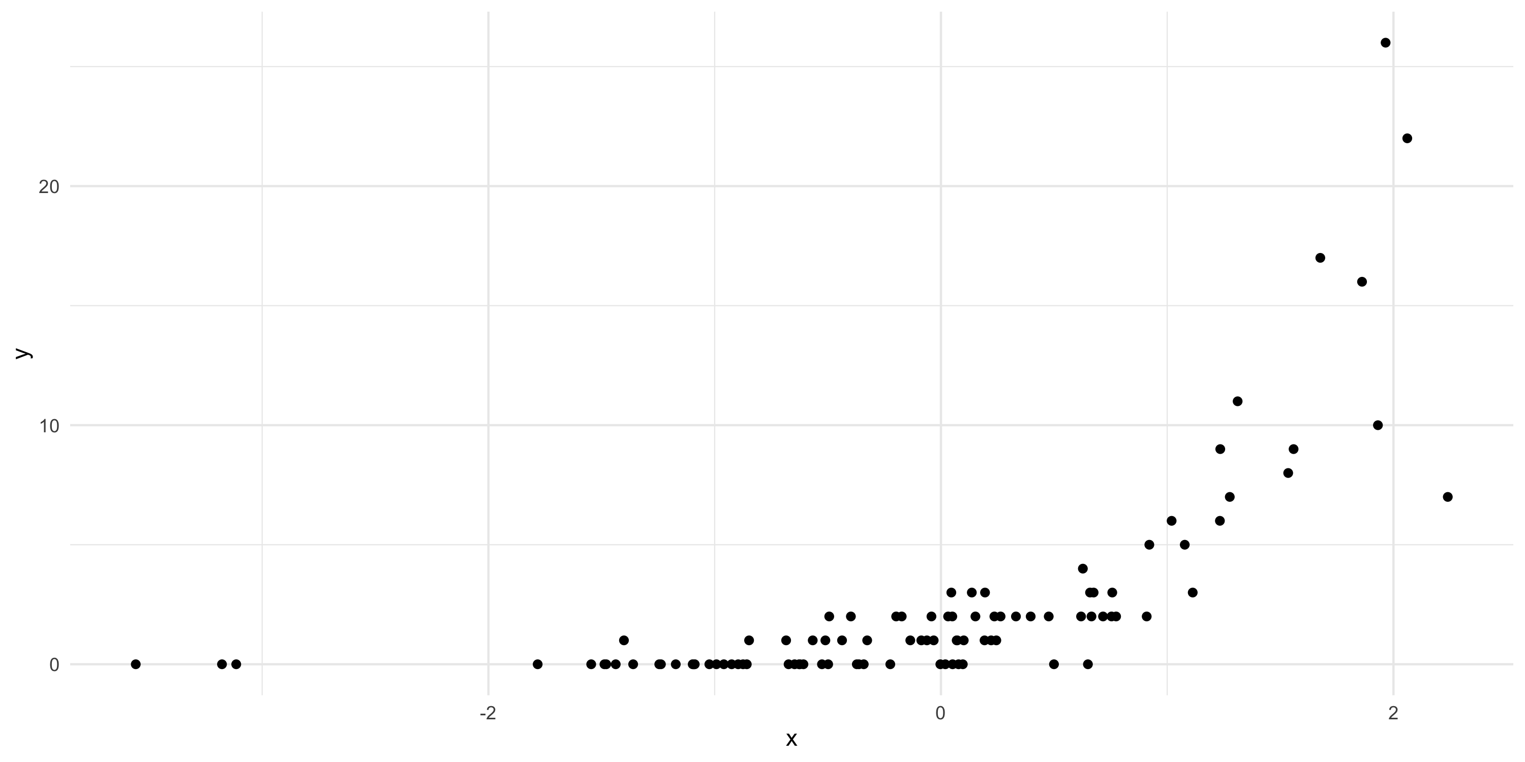
• Assume our model is Y|\beta \sim Poisson(\exp\{ \beta x \}) where x is a covariate
• Assume our prior is \beta \sim N(0, 1)
• Data:

Setting up Metropolis algorithms

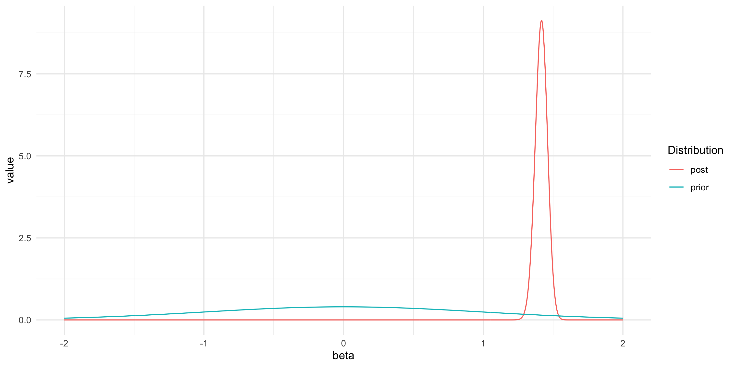
• We are looking for the posterior for \beta that is p(\beta | Y)
• p(\beta | Y) = \frac{p(Y | \beta) p(\beta)}{p(Y)} = \frac{p(Y | \beta) p(\beta)}{\int p(Y|\beta) p(\beta) d\beta}
• We can approximate the posterior numerically because this is an extremely simple problem

beta_vals <- seq(-2, 2, length.out=1000)
delta <- diff(beta_vals)[1]

post_vals_unnorm <- beta_vals %>% sapply(\(beta) exp(sum(dpois(y, exp(x*beta), log=TRUE)) + dnorm(beta, log=TRUE))) 
post_vals <- post_vals_unnorm/sum(post_vals_unnorm)/delta

df_post <- data.frame(beta=beta_vals, post=post_vals, prior=dnorm(beta_vals)) %>%
  tidyr::pivot_longer(cols=c(post,prior))
ggplot(df_post, aes(x=beta, y=value, color=name)) +
  labs(color="Distribution") +
  geom_line() +
  theme_minimal()

Setting up Metropolis algorithms

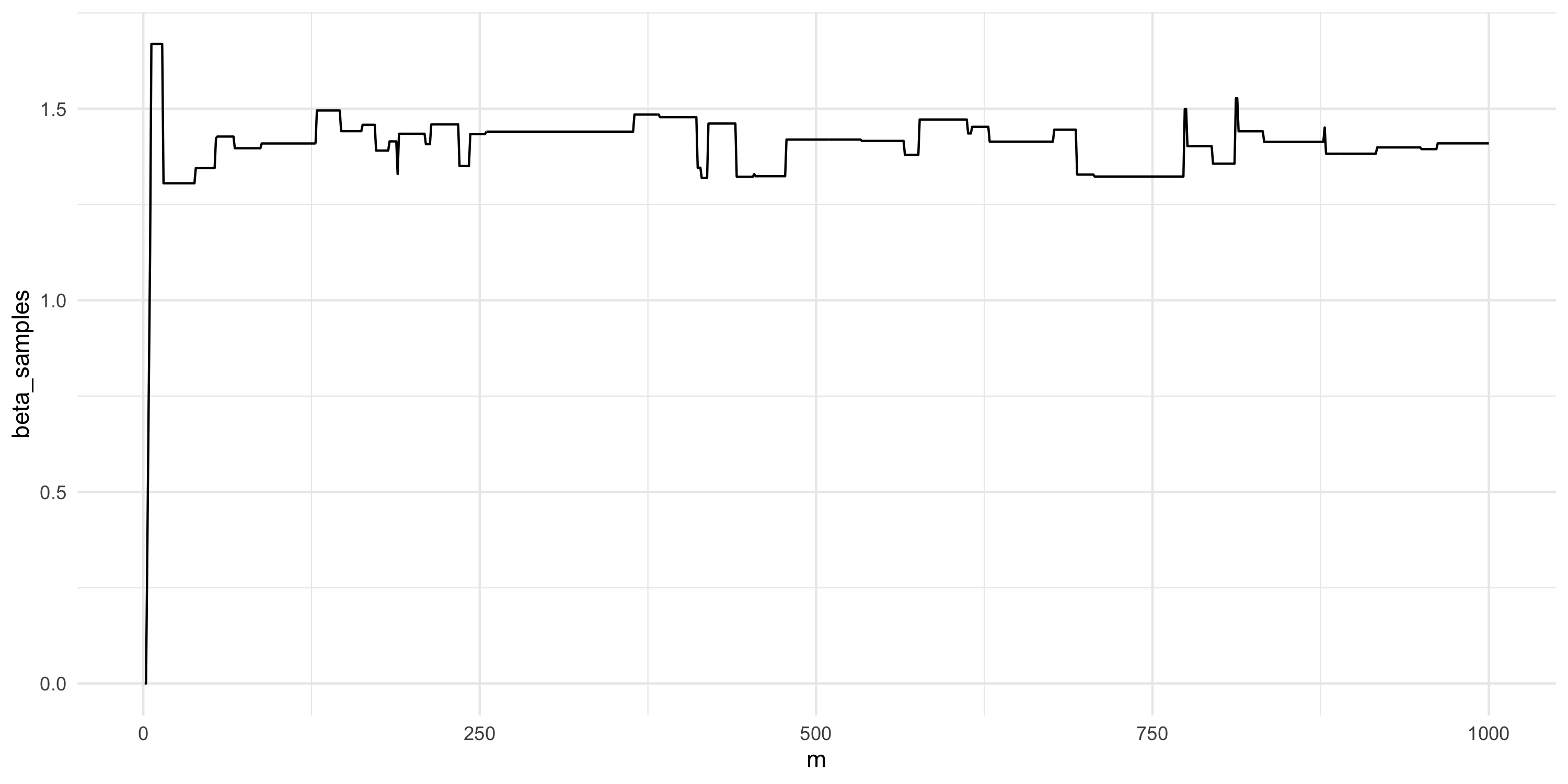
• Let’s try to sample from the posterior using a random walk Metropolis
• i.e., q(\beta | \beta_{\text{current}}) = N(\beta; \beta_{\text{current}}, s^2) for a fixed proposal variance s^2
• i.e., \beta^* = \beta_{\text{current}} + s v where v \sim N(0,1)

n_iter <- 1000
s <- 1

my_rw_metropolis <- function(n_iter, s){
  beta_samples <- rep(NA, n_iter)
  
  beta_samples[1] <- 0 # starting value
  for(m in 2:n_iter){
    
    beta_proposal <- beta_samples[m-1] + s * rnorm(1)
    
    alpha <- sum(dpois(y, exp(x * beta_proposal), log=T)) +
      dnorm(beta_proposal, log=T) -
      sum(dpois(y, exp(x * beta_samples[m-1]), log=T)) -
      dnorm(beta_samples[m-1], log=T)
      
    accept_prob <- min(c(1,exp(alpha)))
    
    U <- runif(1)
    if(U < accept_prob){
      beta_samples[m] <- beta_proposal
    } else {
      beta_samples[m] <- beta_samples[m-1]
    }
  }
  return(beta_samples)
}

beta_samples <- my_rw_metropolis(n_iter, s)

Setting up Metropolis algorithms

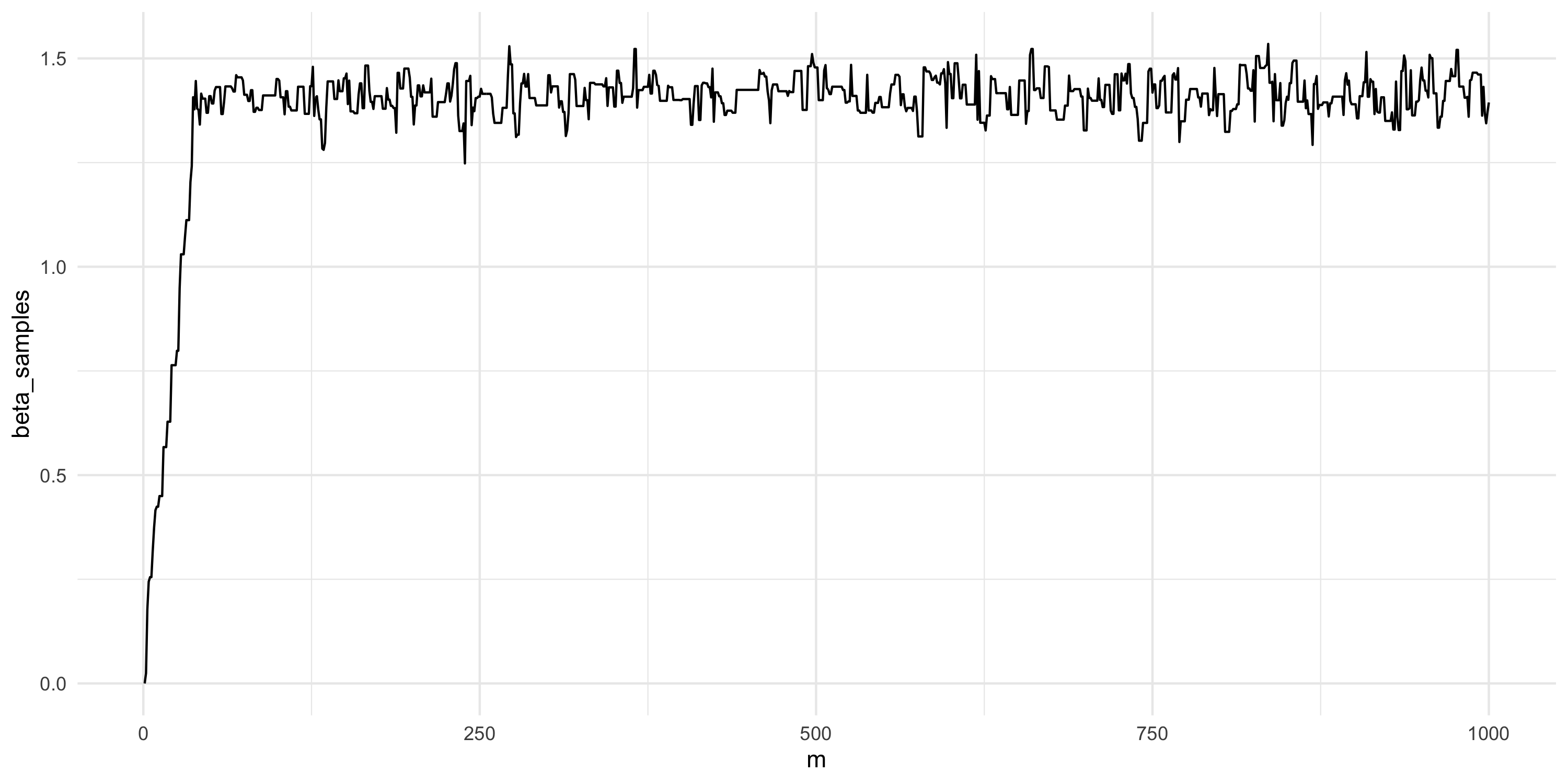
• Comment on this plot. Are you happy with the results? What would you change if not?

Setting up Metropolis algorithms

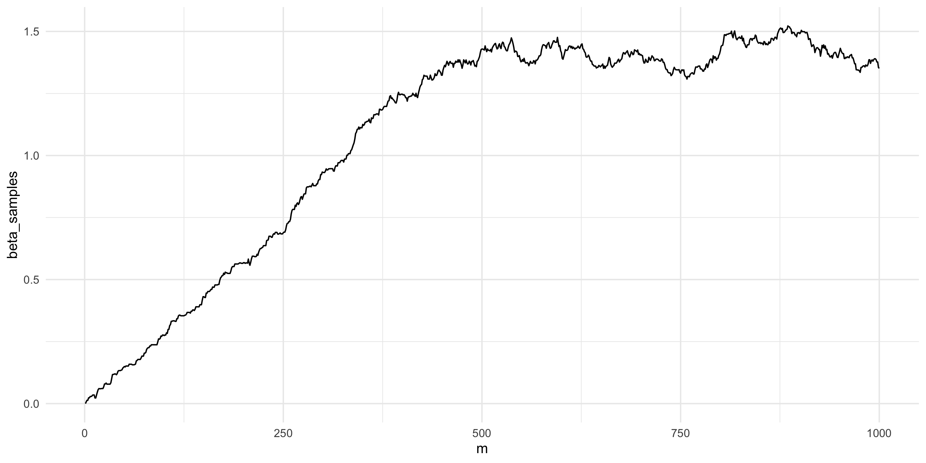
• What about now?

s <- .01

beta_samples <- my_rw_metropolis(n_iter, s)

Setting up Metropolis algorithms

• What about now?

s <- .1

beta_samples <- my_rw_metropolis(n_iter, s)

Setting up Metropolis algorithms

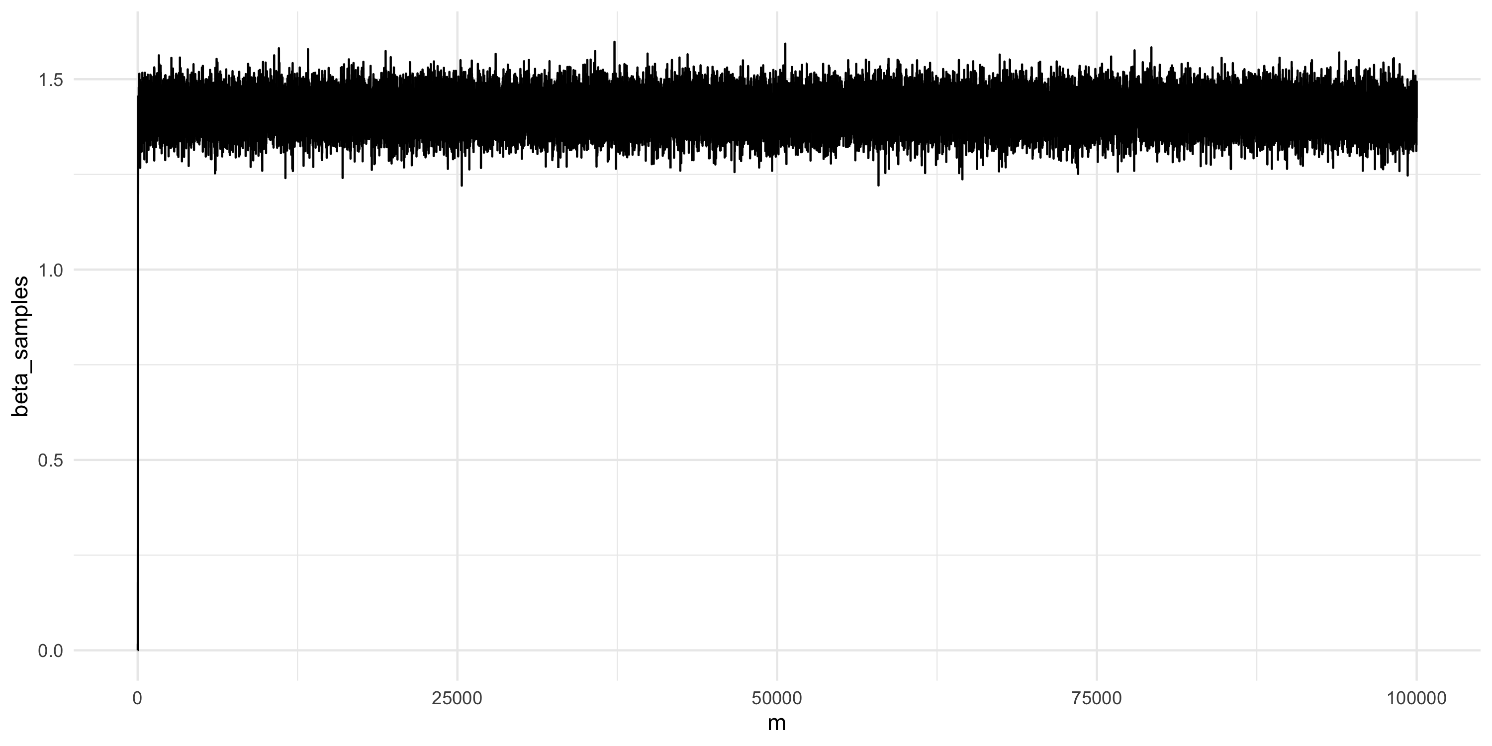
• Let’s run this chain for much longer

s <- .1
n_iter <- 100000

beta_samples <- my_rw_metropolis(n_iter, s)

Setting up Metropolis algorithms

• Drop initial samples as they are burn-in
• Then learn about the posterior by taking summaries
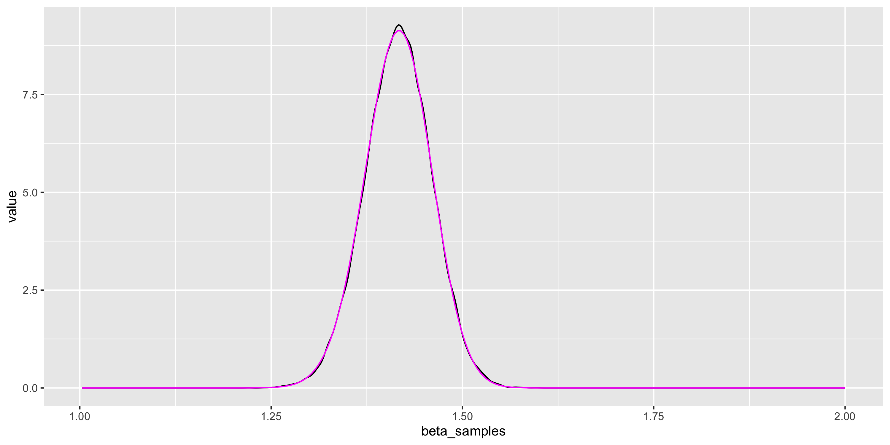
• Example: estimate density using MCMC samples
• Compare with our previous approximation of the posterior (in magenta)

burn_in <- 1000
mcmc_df %>% tail(-burn_in) %>%
  ggplot(aes(beta_samples)) +
  geom_density() +
  geom_line(data=df_post %>% filter(name=="post", beta>1), aes(x=beta, y=value), color="magenta")

More difficult

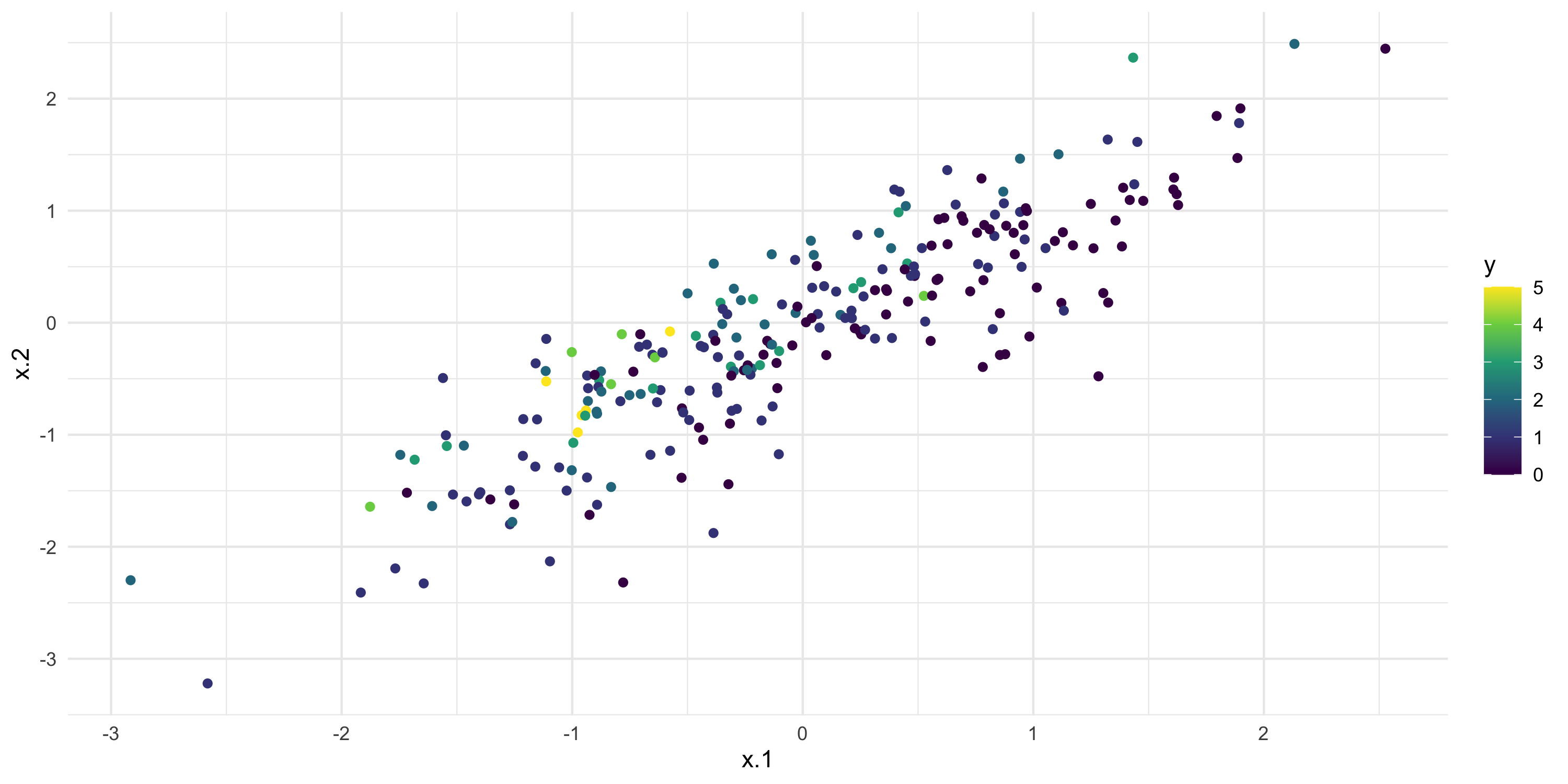
• Now, same problem but the number of predictors is 2 and we make them correlated
• This induces posterior correlation on their regression coefficients

Numerical approximation of the 2D posterior

• We do the same thing as before, but now we work in 2 dimensions
• We let \beta \sim N(0, I_2) be our prior

beta_vals <- expand.grid(b1vals <- seq(-2, 0, length.out=500),
                         b2vals <- seq(0, 2, length.out=500))
colnames(beta_vals) <- c("beta.1", "beta.2") 
delta <- diff(b1vals)[1]^2

post_vals_unnorm <- beta_vals %>% apply(1, \(beta) exp(sum(dpois(y, exp(X %*% beta), log=TRUE)) + sum(dnorm(beta, log=TRUE)))) 
post_vals <- post_vals_unnorm/sum(post_vals_unnorm)/delta

df_post <- data.frame(beta_vals, post=post_vals)

ggplot(df_post, aes(x=beta.1, y=beta.2, fill=post)) +
  labs(fill="Posterior") +
  geom_raster() +
  scale_fill_scico(palette="davos", direction=-1) +
  theme_minimal()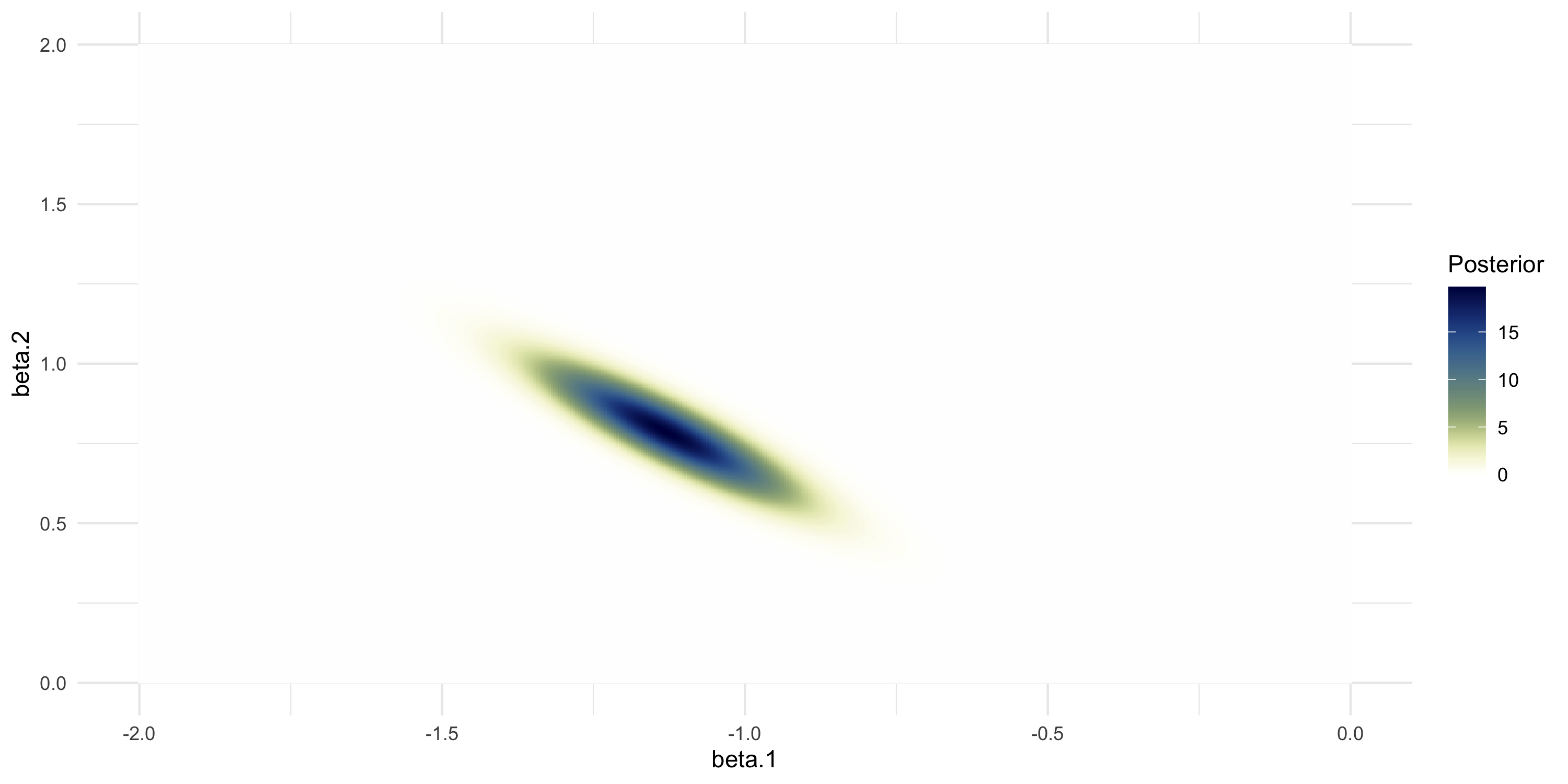

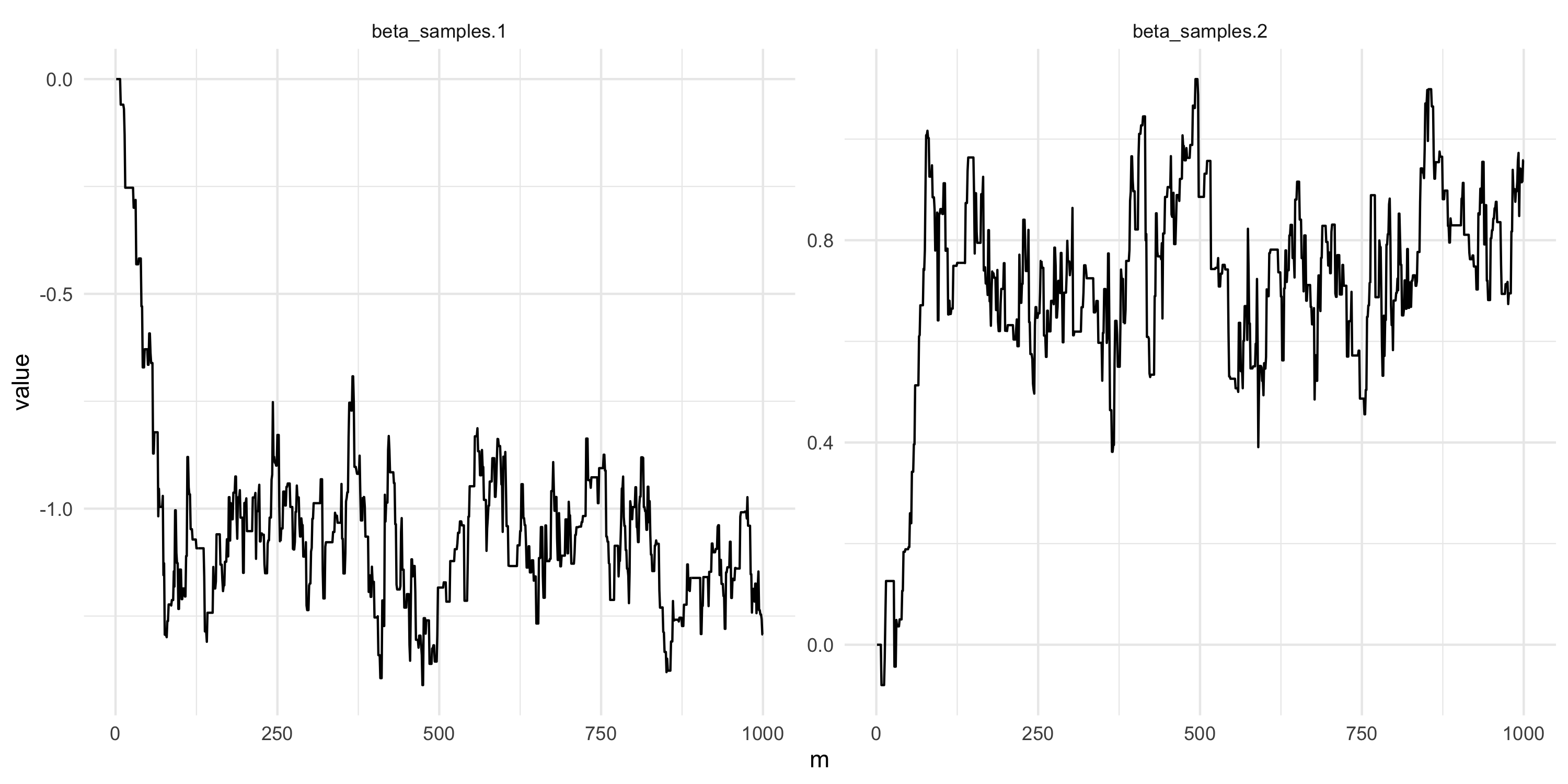
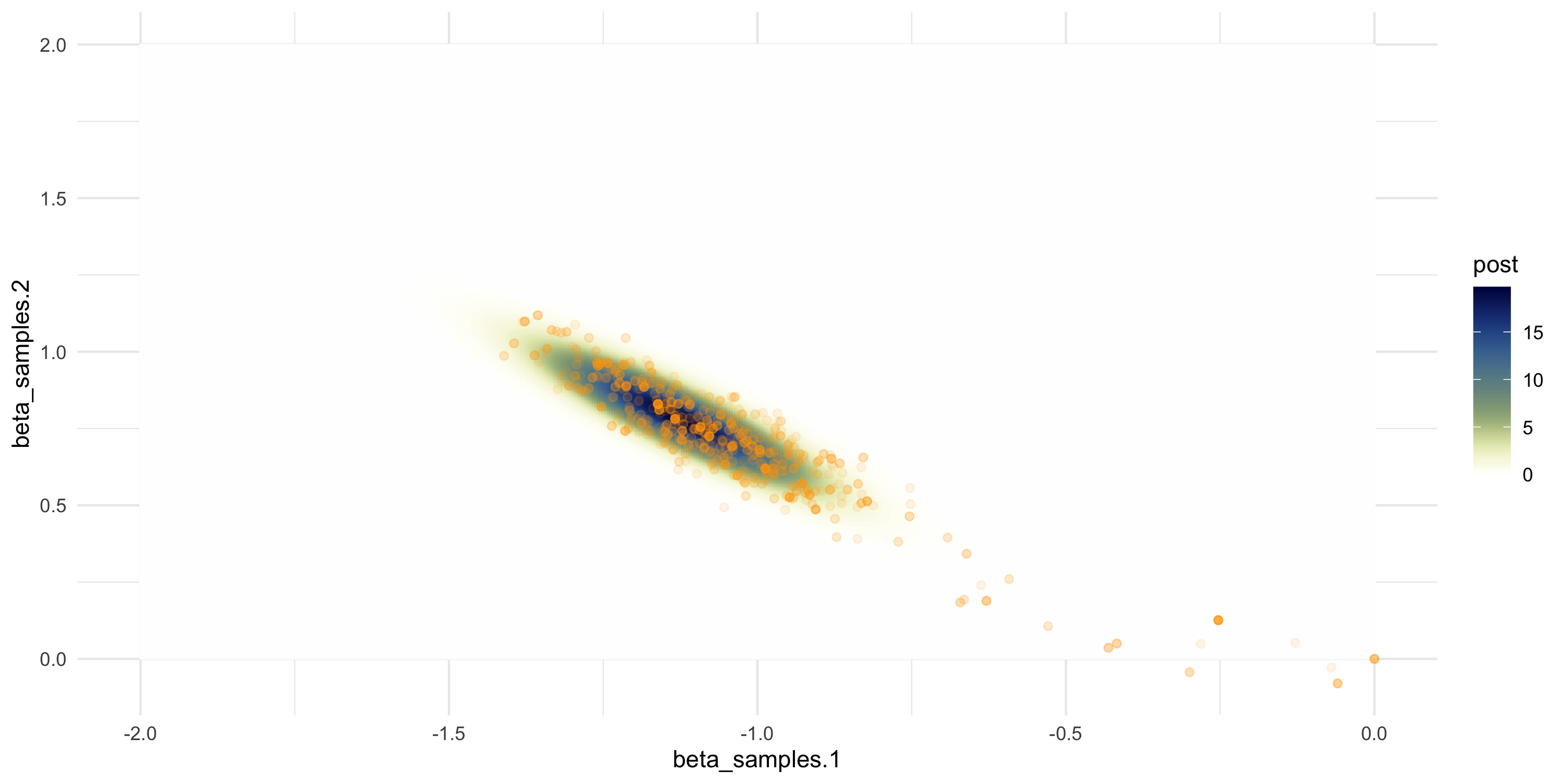
Setting up random walk Metropolis

• We just change the previous code to calculate likelihoods and priors

my_rw_metropolis <- function(n_iter, s){
  beta_samples <- matrix(NA, nrow=n_iter,ncol=ncol(X))
  
  beta_samples[1,] <- 0 # starting value
  for(m in 2:n_iter){
    
    beta_proposal <- beta_samples[m-1,] + rnorm(2) * s
    
    alpha <- sum(dpois(y, exp(X %*% beta_proposal), log=T)) +
      sum(dnorm(beta_proposal, log=T)) -
      sum(dpois(y, exp(X %*% beta_samples[m-1,]), log=T)) -
      sum(dnorm(beta_samples[m-1,], log=T))
      
    accept_prob <- min(c(1,exp(alpha)))
    
    U <- runif(1)
    if(U < accept_prob){
      beta_samples[m,] <- beta_proposal
    } else {
      beta_samples[m,] <- beta_samples[m-1,]
    }
  }
  return(beta_samples)
}

Setting up random walk Metropolis

s <- .1
n_iter <- 1000

beta_samples <- my_rw_metropolis(n_iter, s)

Setting up random walk Metropolis

Adaptive Metropolis algorithms

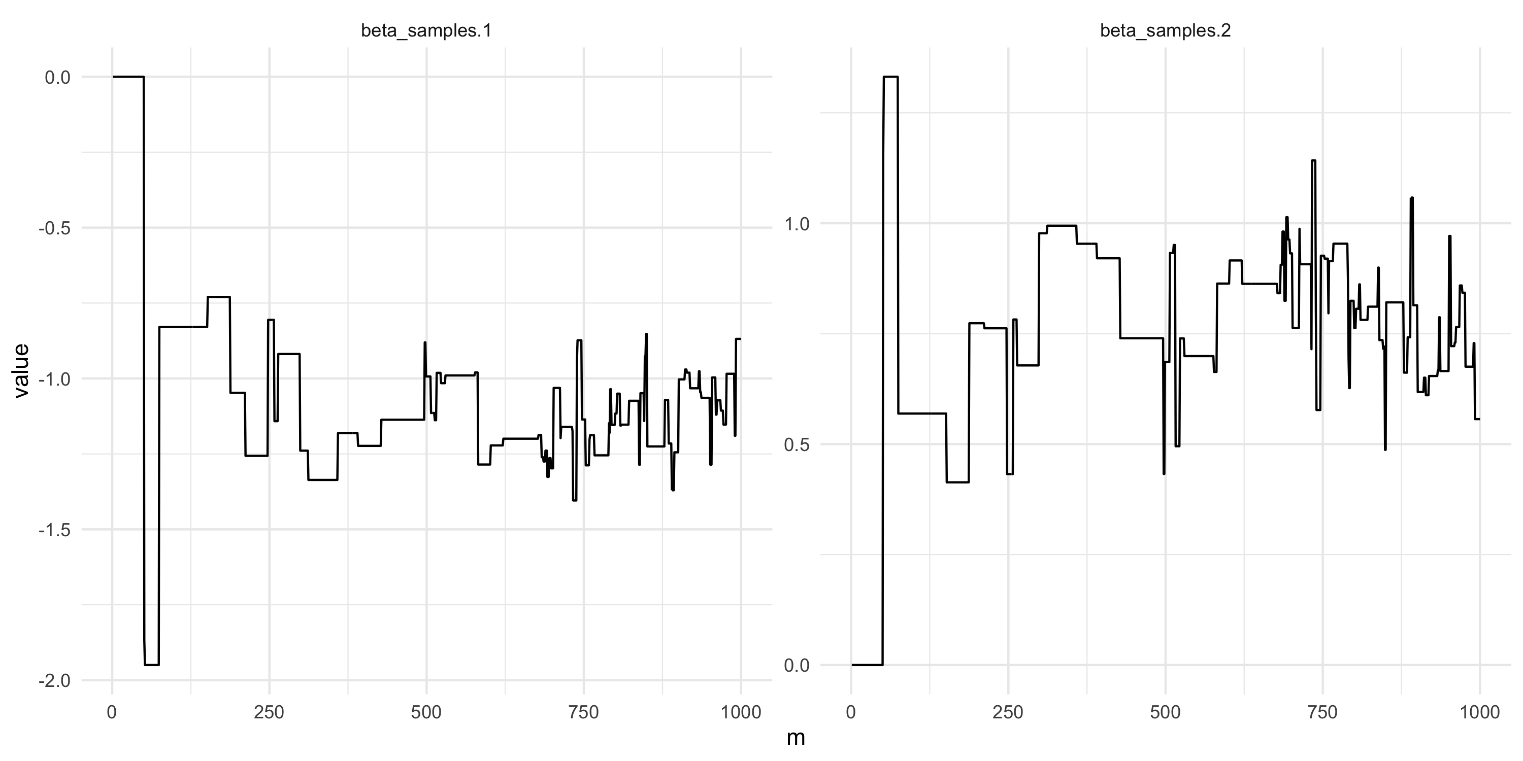
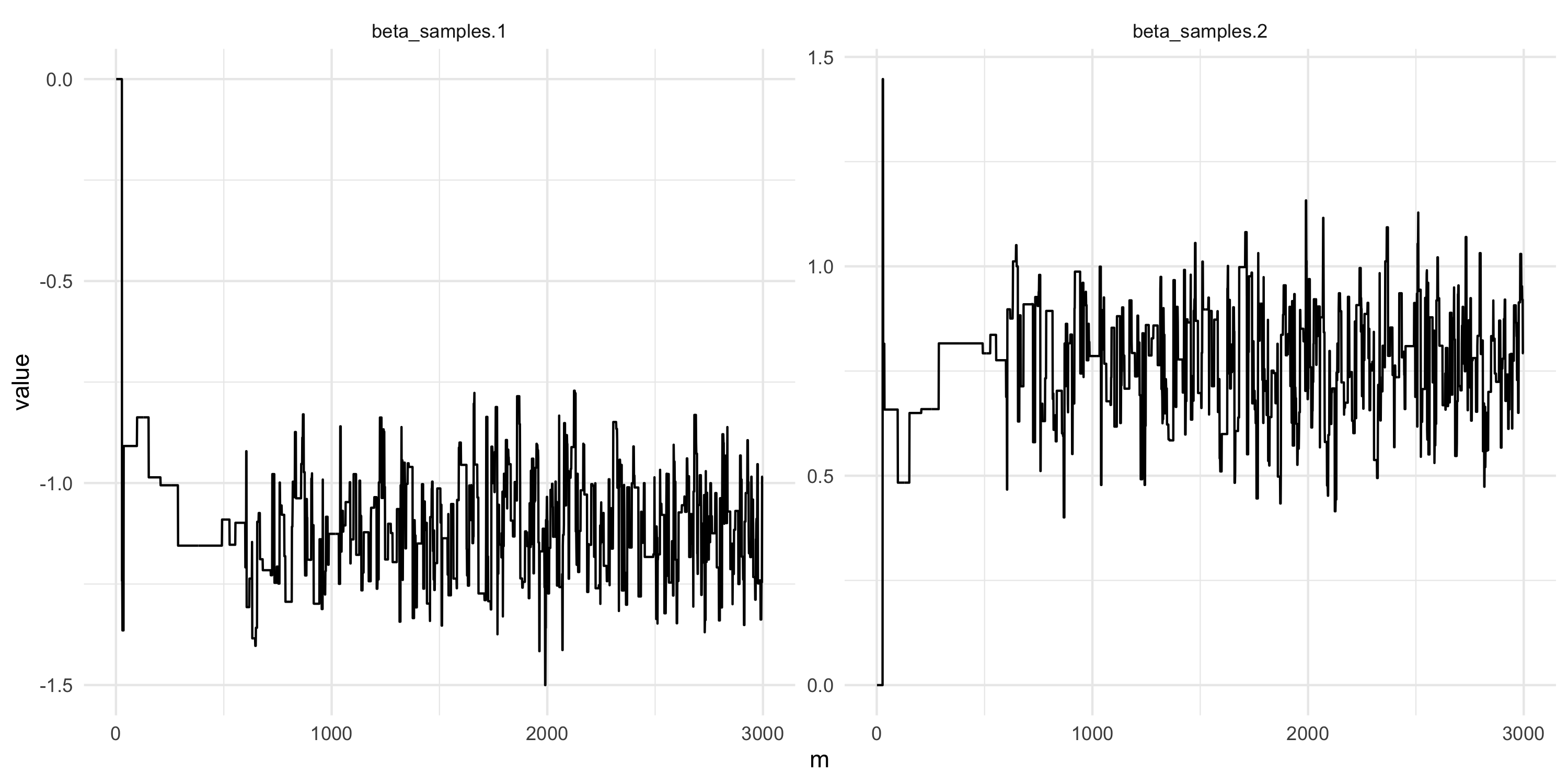
• Tuning the proposal so it behaves nicely can be tedious
• This can be made automatic via adaptive Metropolis algorithms
• I am providing you with source code to run adaptive Metropolis
• This is a modification of adaptMCMC::MCMC. Runs Robust Adaptive Metropolis, Vihola (2012)
• Includes Jacobian adjustment

source("code/adaptive_MCMC_mod.R")

mypost <- function(beta){
  sum(dpois(y, exp(X %*% beta), log=T)) + sum(dnorm(beta, log=TRUE))
}

adaptive_out <- MCMCmod(mypost, n_iter <- 1000, c(0, 0), cbind(c(-10,-10), c(10,10)), acc.rate = 0.25)

Adaptive Metropolis algorithms

adaptive_out <- MCMCmod(mypost, n_iter <- 3000, c(0, 0), cbind(c(-10,-10), c(10,10)), acc.rate = 0.25)

Analyzing MCMC output

• We can use package coda for MCMC convergence analysis and other MCMC tools
• Convergence analysis is based on output from multiple runs of MCMC

library(coda)

n_iter <- 1000
run_1 <- MCMCmod(mypost, n_iter, c(0, 0), cbind(c(-10,-10), c(10,10)), acc.rate = 0.25)$samples %>% as.mcmc()
run_2 <- MCMCmod(mypost, n_iter, c(0, 0), cbind(c(-10,-10), c(10,10)), acc.rate = 0.25)$samples %>% as.mcmc()

(analyse_converg <- gelman.diag(list(run_1, run_2)))

Potential scale reduction factors:

     Point est. Upper C.I.
[1,]       1.25       1.82
[2,]       1.07       1.28

Multivariate psrf

1.21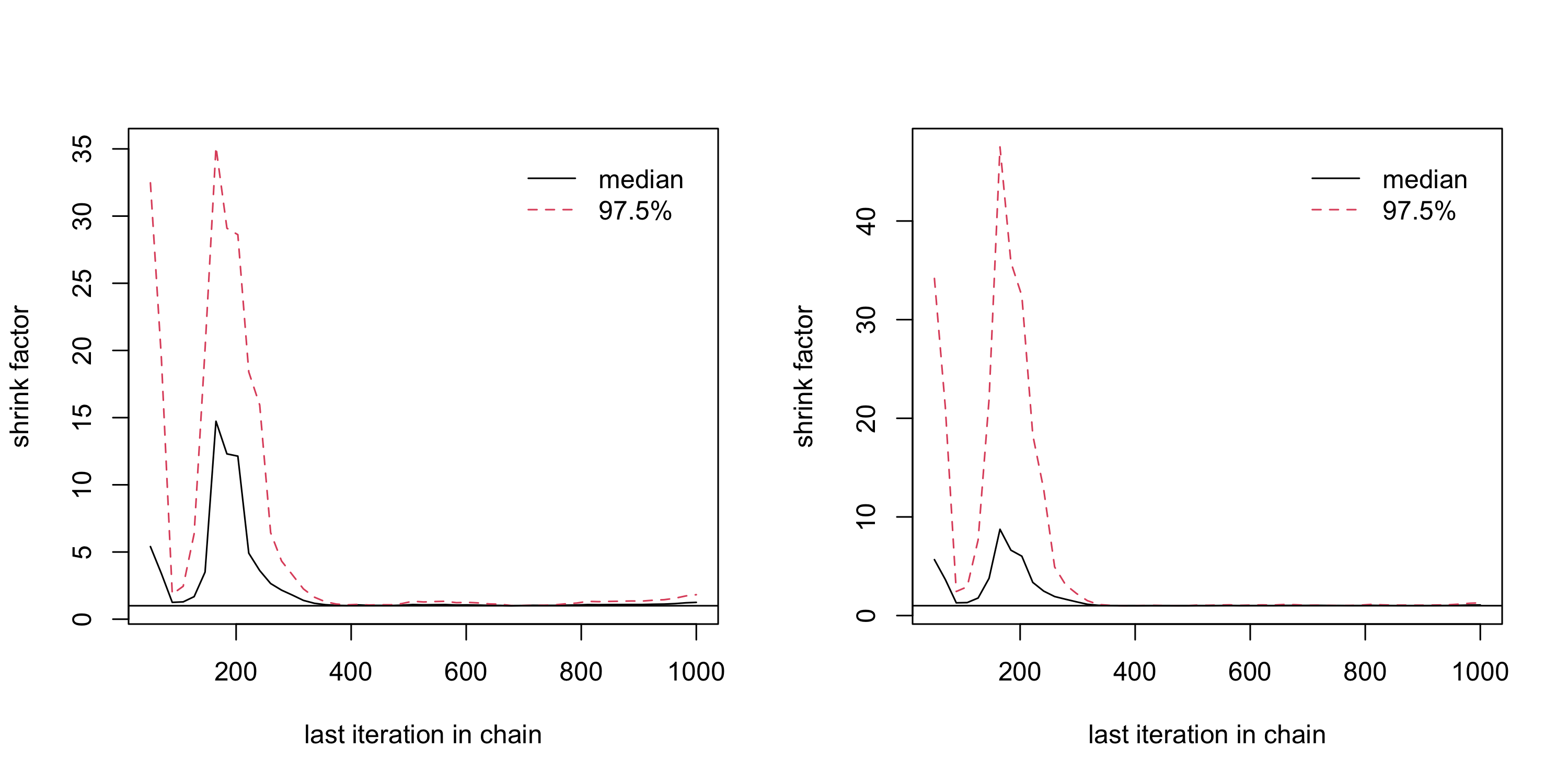

gelman.plot(list(run_1, run_2))

Analyzing MCMC output

• We can use package coda for MCMC convergence analysis and other MCMC tools
• Convergence analysis is based on output from multiple runs of MCMC

n_iter <- 20000
run_1 <- MCMCmod(mypost, n_iter, c(0, 0), cbind(c(-10,-10), c(10,10)), acc.rate = 0.25)$samples %>% 
  head(-n_iter/2) %>% as.mcmc()
run_2 <- MCMCmod(mypost, n_iter, c(0, 0), cbind(c(-10,-10), c(10,10)), acc.rate = 0.25)$samples %>% 
  head(-n_iter/2) %>% as.mcmc()

(analyse_converg <- gelman.diag(list(run_1, run_2)))

Potential scale reduction factors:

     Point est. Upper C.I.
[1,]       1.00       1.02
[2,]       1.01       1.02

Multivariate psrf

1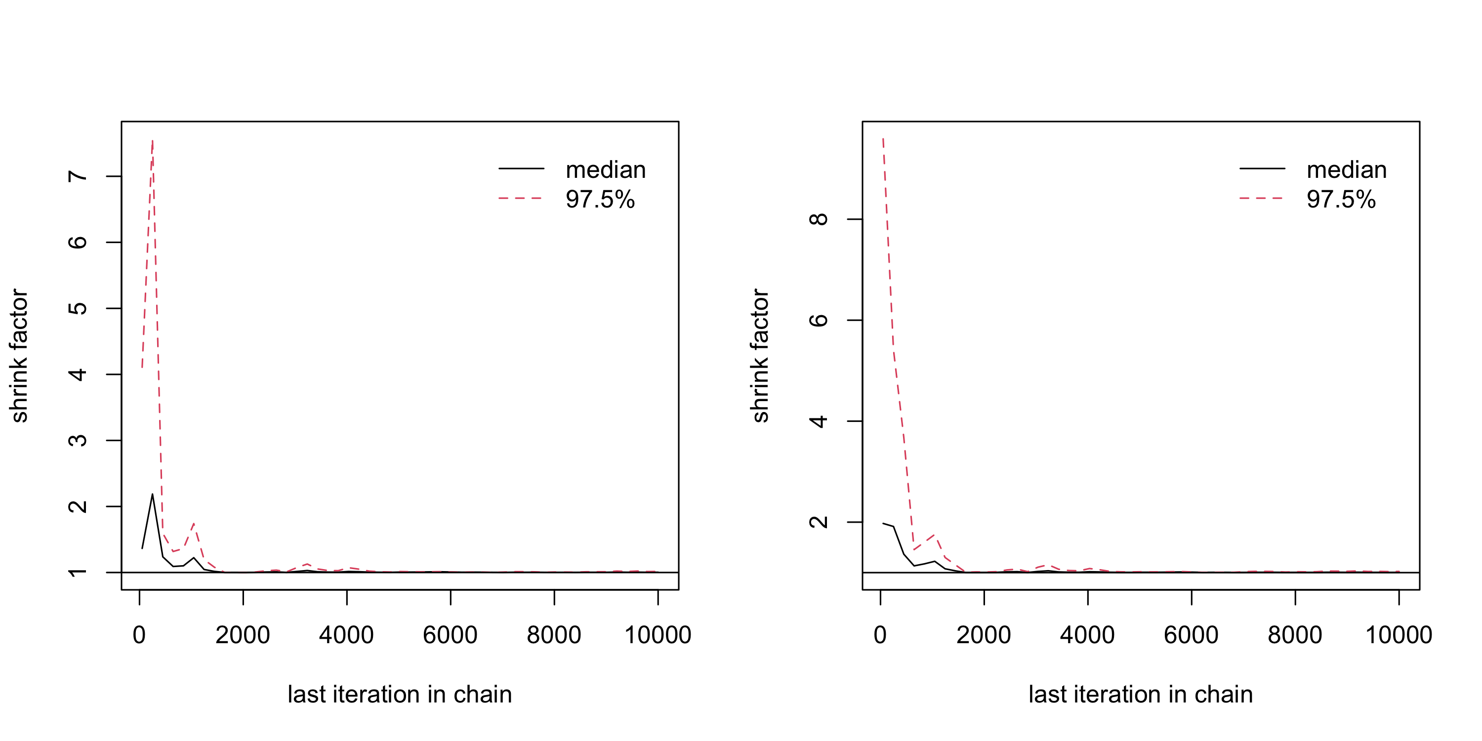

gelman.plot(list(run_1, run_2))

Analyzing MCMC output

• Because MCMC gives us correlated sample, the quality of the sample is lower when there is high autocorrelation in the chain
• We can compute the Effective Sample Size, that is the size of an independent sample equivalent to our correlated sample
• Typically, if we have T samples from MCMC, the effective size is smaller, sometimes much smaller!
• See for example in our case:

eff_size <- (run_1 %>% effectiveSize())

• We had run the chain for 20000 iterations and removed the first 10000 as burn-in, but our sample is equivalent to an independent sample of size 947.1310064, 933.3870376

Postprocessing MCMC output

• Suppose we have a sample \{ \theta_t \}_{t=1}^T obtained from MCMC
• Assume everything checks out in terms of convergence, so \{ \theta_t \}_{t=1}^T \sim p(\theta | Y)
• Estimating posterior summaries? Use the MCMC sample
• Example. Estimate Pr(\theta > 0.9 | Y) using MCMC output:

\hat{Pr}(\theta > 0.9 | Y) = \frac{\sum_{t}^{T} 1_{\{\theta_t > 0.9\} }}{T}

• In R, mean(theta_mcmc_sample > 0.9)
• Notice Pr(\theta > 0.9 | Y) = E(1_{ \{ \theta > 0.9 \} } | Y) and we are computing this expectation via a sample mean
• This is just like any Monte Carlo approximation

Back to spatial models

• Full Bayesian inference may involve MCMC algorithms
• Large number of iterations may be required for satisfactory ability in summarizing the posterior
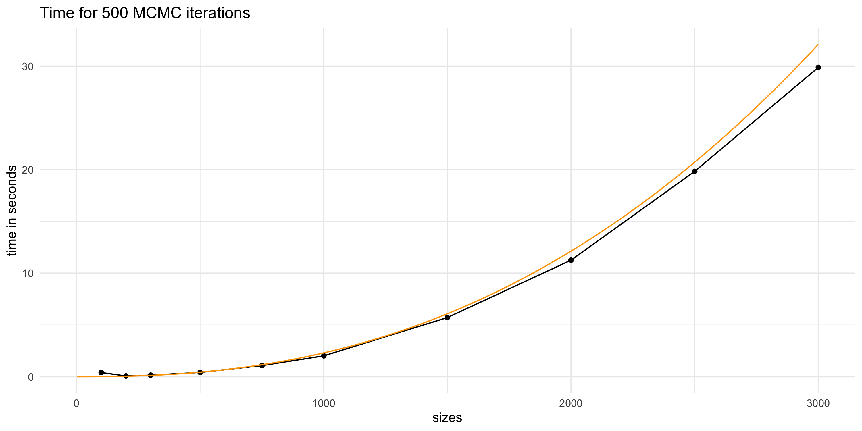
• Spatial models based on GPs scale poorly with data dimension
• ie. double the data size, (much) more than double the computation requirement
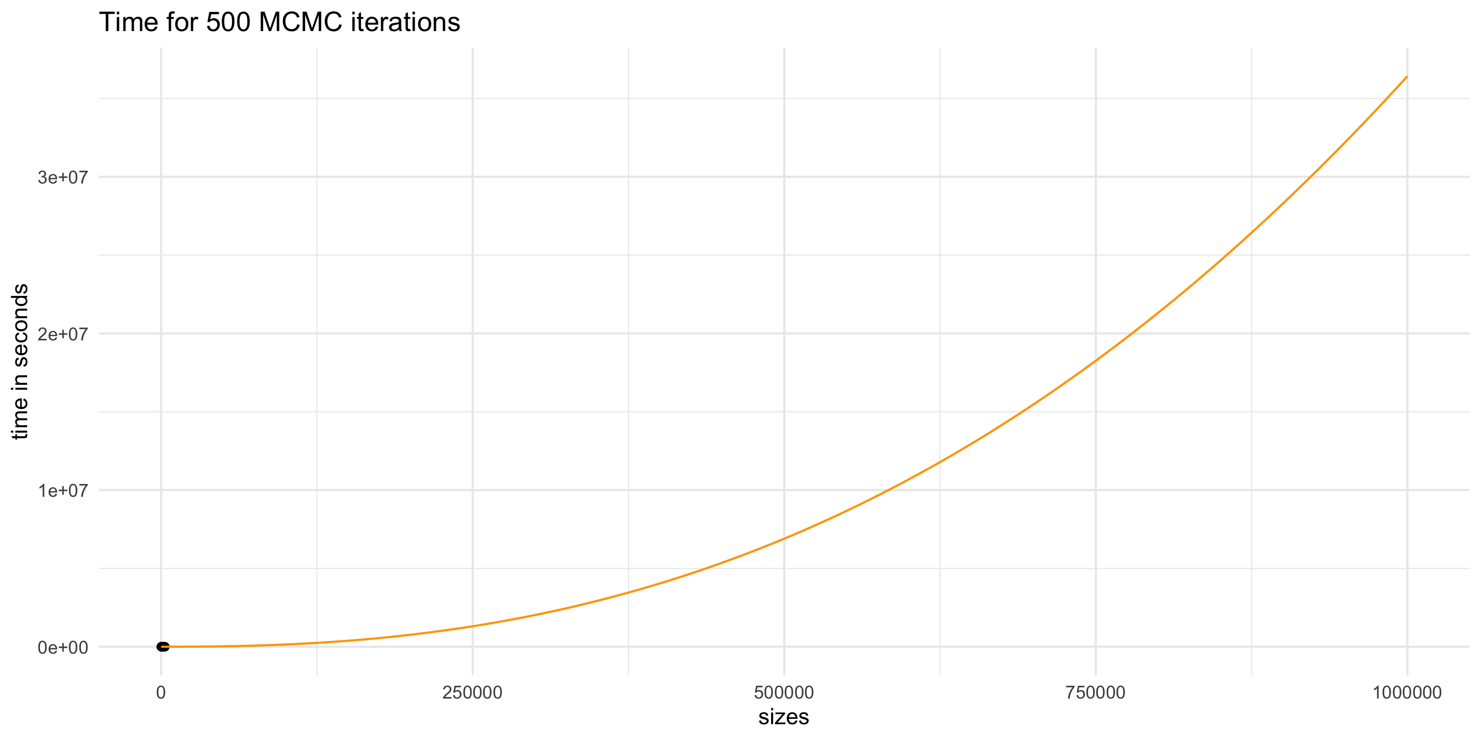
• Running MCMC for many iterations when each of them is slow? Do we have time for everything?

Projecting compute time for GP models

Projecting compute time for GP models

Projecting compute time for GP models

• If our dataset had n=10^6 then we could perform 500 MCMC iterations in no less than 8333 hours (about 1 year)
• A single run of MCMC on 25000 iterations would then take 50 years
• Assuming our compute power will increase does not help
• Data sizes and complexity will also presumably increase in time

Computational complexity

• We can measure the theoretical complexity of a model based on
• Memory requirements: how much storage we need to build the model and run operations
• Flops: the number of CPU operations that are necessary for running our algorithms
• Time: the amount of time for running our algorithms

Memory requirements

• This is one component of computational complexity
• How much memory do we need to work with GPs?
• Suppose data size is n
• Then, at a minimum, we could have this model:

Y_{\cal L} \sim N(0, C_{\theta})

• Because we need to do operations with C_{\theta}, we need to store it in memory
• C_{\theta} has dimension n \times n and is symmetric with a constant diagonal (typically)
• We thus need to store at least n (n-1) + 1 values
• This assumes we have algorithms that can take advantage of structure in C_{\theta}
• Otherwise, we need to store n^2 elements
• For large n, the numbers n (n-1) + 1 = n^2 - n + 1 and n^2 are the same order of magnitude
• In both cases, we say O(n^2) is the memory storage requirement

Flops

• In the algorithms we have considered we typically need to perform 2 basic operations
  1. Evaluation of multivariate Gaussian density
  2. Sampling from a multivariate Gaussian density
• The cost in flops (number of operations) of the main operations we need in both cases is computed as
  1. If A is (n \times m) and B is (m \times p) then computing AB costs O(nmp)
  2. If A is symmetric positive definite of size (n \times n), then chol(A) costs O(n^3)
  3. If L is lower triangular of size (n \times n), then L^{-1} costs O(n)

Evaluation of multivariate Gaussian

• Recall: p(x; \mu, \Sigma) = |2\pi \Sigma |^{-\frac{1}{2}} \exp\left\{ -\frac{1}{2}(x - \mu)^T \Sigma^{-1} (x - \mu) \right\}

• Cholesky decomposition of \Sigma: it is the lower triangular matrix L such that L L^T = \Sigma

• With L, we do \Sigma^{-1} = L^{-T} L^{-1} where L^{-T} = (L^{-1})^T and det(\Sigma) = 2 \prod_{i=1}^n L_{ii}

\log p(x; \mu, \Sigma) = -\frac{n}{2} \log(2\pi) - \sum_{i=1}^n\log(L_{ii}) - \frac{1}{2}(x-\mu)^T L^{-T} L^{-1} (x-\mu)

1. Cost of getting L: \quad O(n^3)
2. Cost of x^* = (x-\mu)^TL^{-T}: \quad O(n^2)
3. Cost of \sum \log \{L_{ii}\} and x^* x^{*^T}: \quad O(n)

Overall cost: O(n^3). This is quite terrible!

Sampling of multivariate Gaussian

• Recall: if Z \sim N(0,I_n) then X = a + LZ \sim N(a, LL^T)
• If we want to sample Y \sim N(0, C):
  1. Compute $L = $chol(C). (In R, L = t(chol(C)))
  2. Sample Z \sim N(0,I_n)
  3. Compute Y = L Z

Budget:
(1) Cost of getting L: \quad O(n^3) (2) Cost of sampling Z is the same as n times the cost of sampling V \sim N(0,1): \quad O(n) (3) Cost of getting Y: \quad O(n^2)

Overall cost O(n^3). Once again, not scalable to large n.

Back to spatial models

• Full Bayesian inference may involve MCMC algorithms requiring mv Gaussian density evaluation and sampling
• Spatial models based on GPs scale O(n^3) with data dimension
• ie. double the data size, (much) more than double the computation requirement
• Running MCMC for many iterations when each of them is slow? Do we have time for everything?

We have not considered another important point:

• How many iterations do we need for MCMC to converge?
• How many iterations do we need to collect an effective sample of good size?
• MCMC convergence depends on dimension of the posterior and the degree of posterior dependence
• Flops and memory are only giving us a partial picture
• We need fast computations before we can even consider MCMC convergence issues