Point-referenced spatial data
Spatial Statistics - BIOSTAT 696/896
University of Michigan
Recap: point-referenced spatial data
- We observe Y(s) at location s
- What is s in this case?
- What are some examples of point-referenced data?
Point-referenced spatial data
- Observe Y(s) at s \in \cal L = \{s_1, \dots, s_n\}
- The set \cal L is assumed fixed and known, ie the locations are not random
Goals
- Learn/estimate how Y(\cdot) changes in space. Model the spatial dependence
- Generalize linear regression: drop i.i.d. assumption in favor of spatial dependence
- Predict Y(\cdot) at locations that were not observed
Example
- How does air pollution spread geographically?
- Considering the impact of air pollution on health, how should we model the spread of respiratory disease?
- Using a fixed set of observations of air pollution, how can we estimate the level of air pollution everywhere else?
Exploratory analysis and simulation
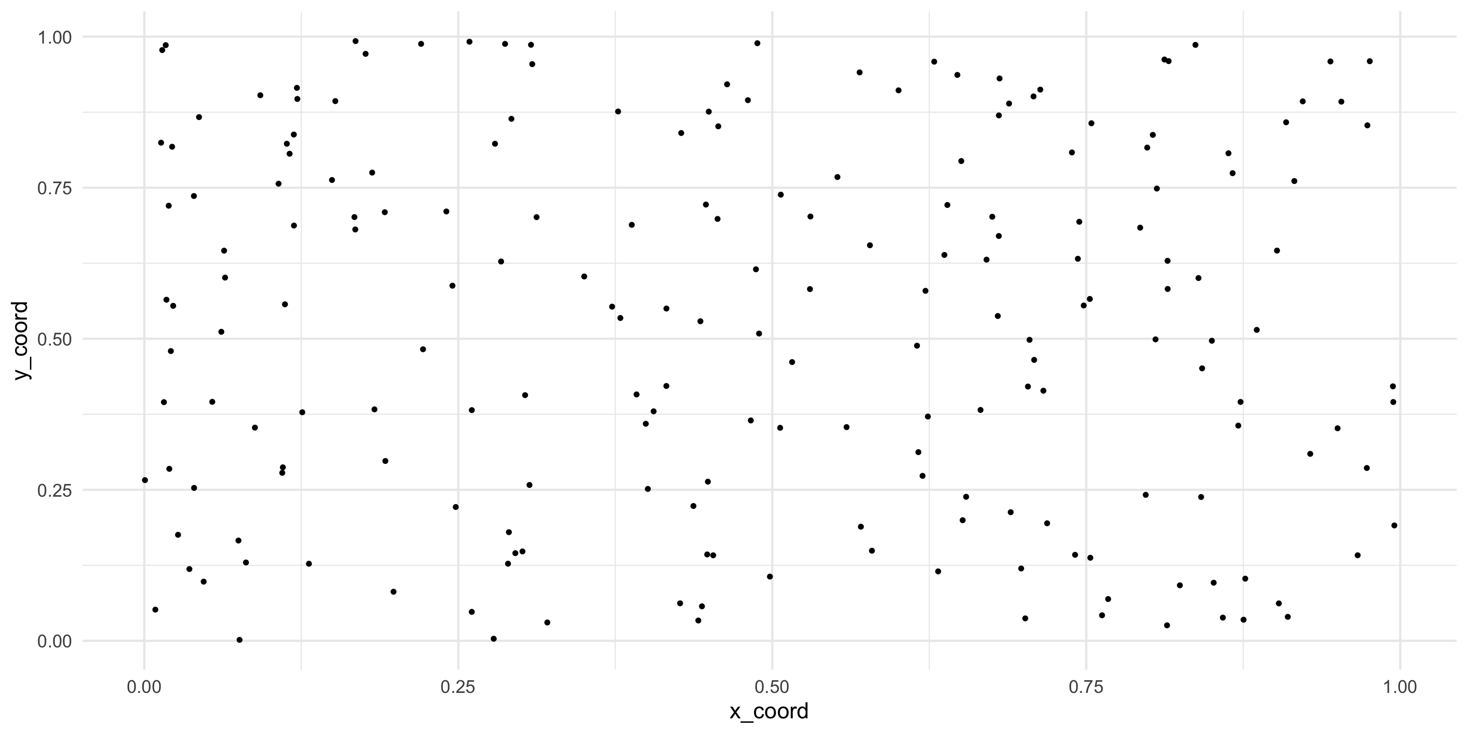
- Simulating a fixed set of spatial locations
- This is just for simulation. Remember with point-referenced data the coordinates are given and non-random
- Remember to set the seed for reproducible analyses!!
Plotting
Exploratory analysis and simulation
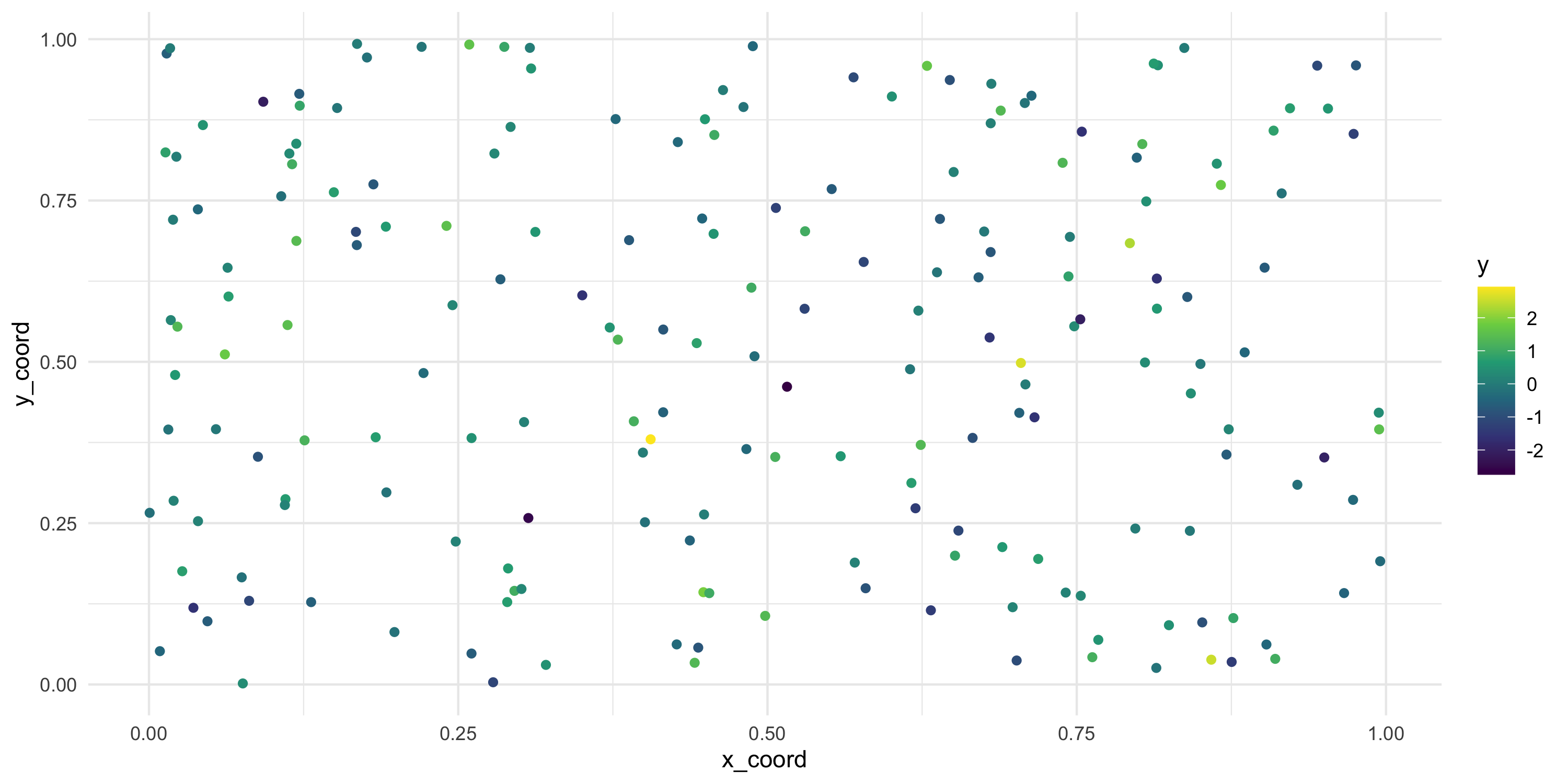
- We just have locations now, there is no data. Let’s generate some data for those locations
- No need to set the seed here. The script will run from the beginning and do all RNGs in sequence
- You can set the seed here if you expect to run chunks of code in different sequences
- How many random variables are we generating?
- What do you expect to see when we plot
yon the coordinates we had before? Why?
Exploratory analysis and simulation
Exploratory analysis and simulation
Make it easier to see there is no spatial dependence by
- increasing sample size
Exploratory analysis and simulation
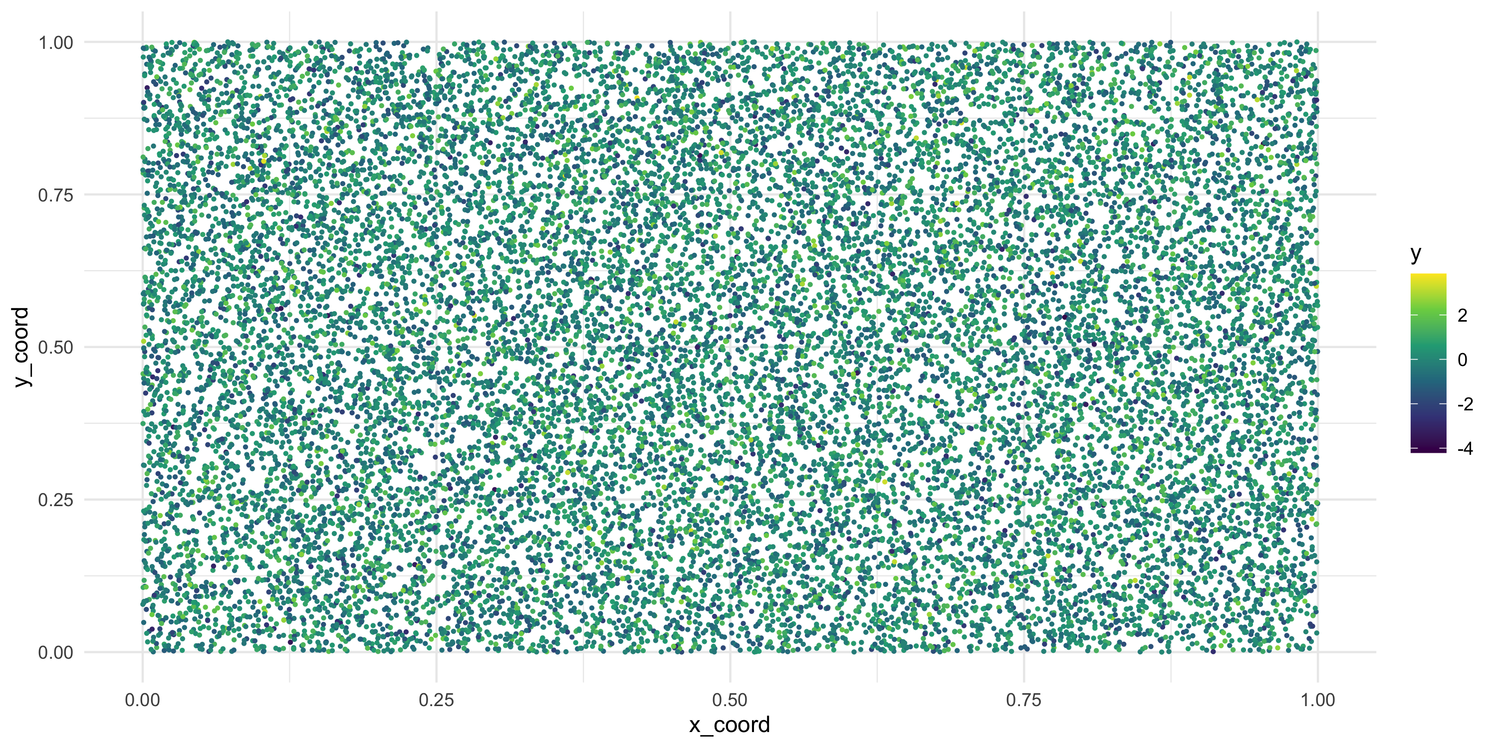
Make it easier to see there is no spatial dependence by
- plotting on a regular grid of spatial locations
- regular grid = each data point can be plotted as a pixel on a raster image
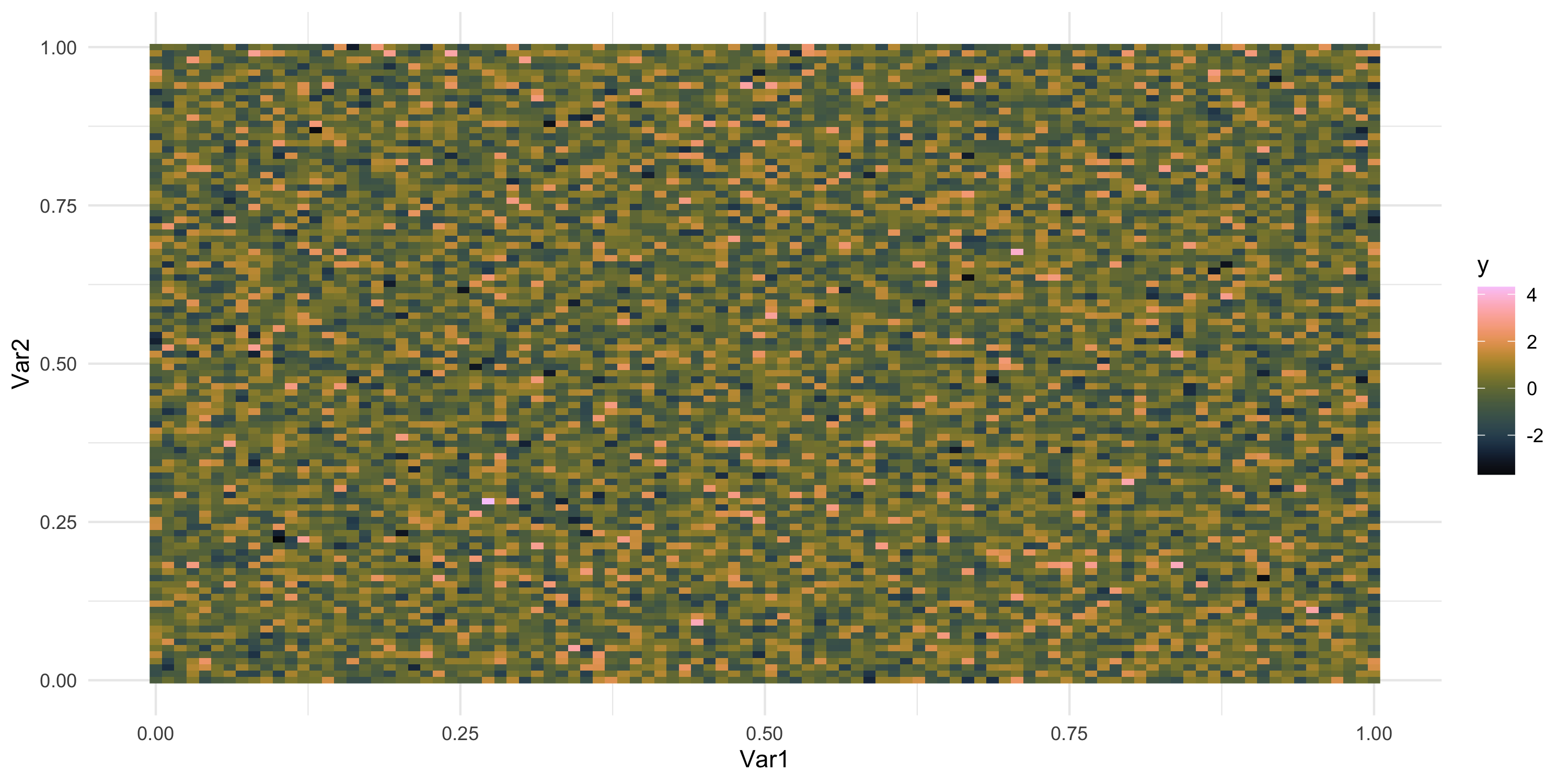
Exploratory analysis and simulation
- We have seen simulated spatial data without spatial dependence
- What would we expect to see if there was spatial dependence?
- Can you think of ways we could simulate data with spatial dependence?
Exploratory analysis and simulation
- What does spatial dependence “look like”? Example 1
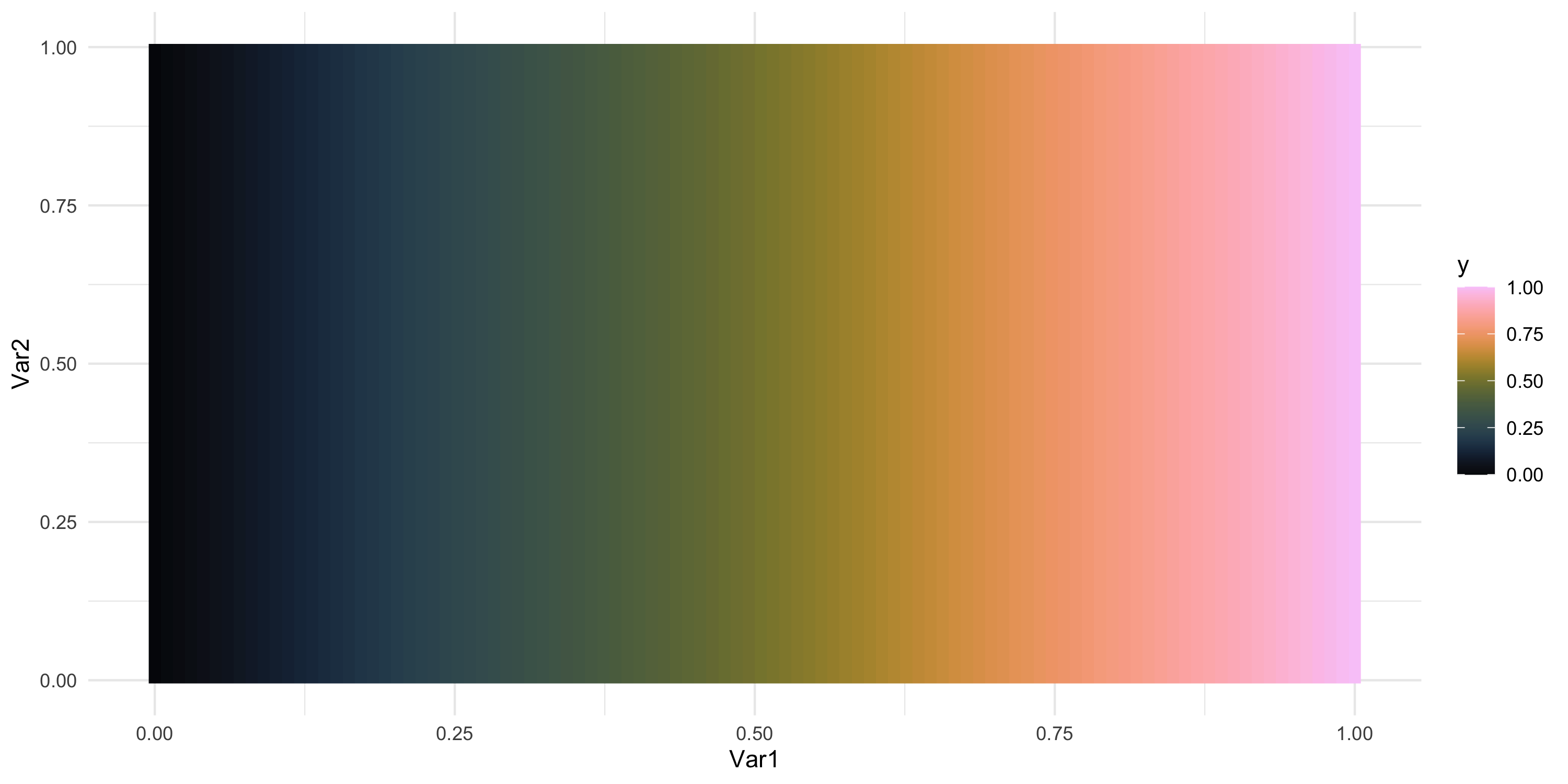
Exploratory analysis and simulation
- What does spatial dependence “look like”? Example 2
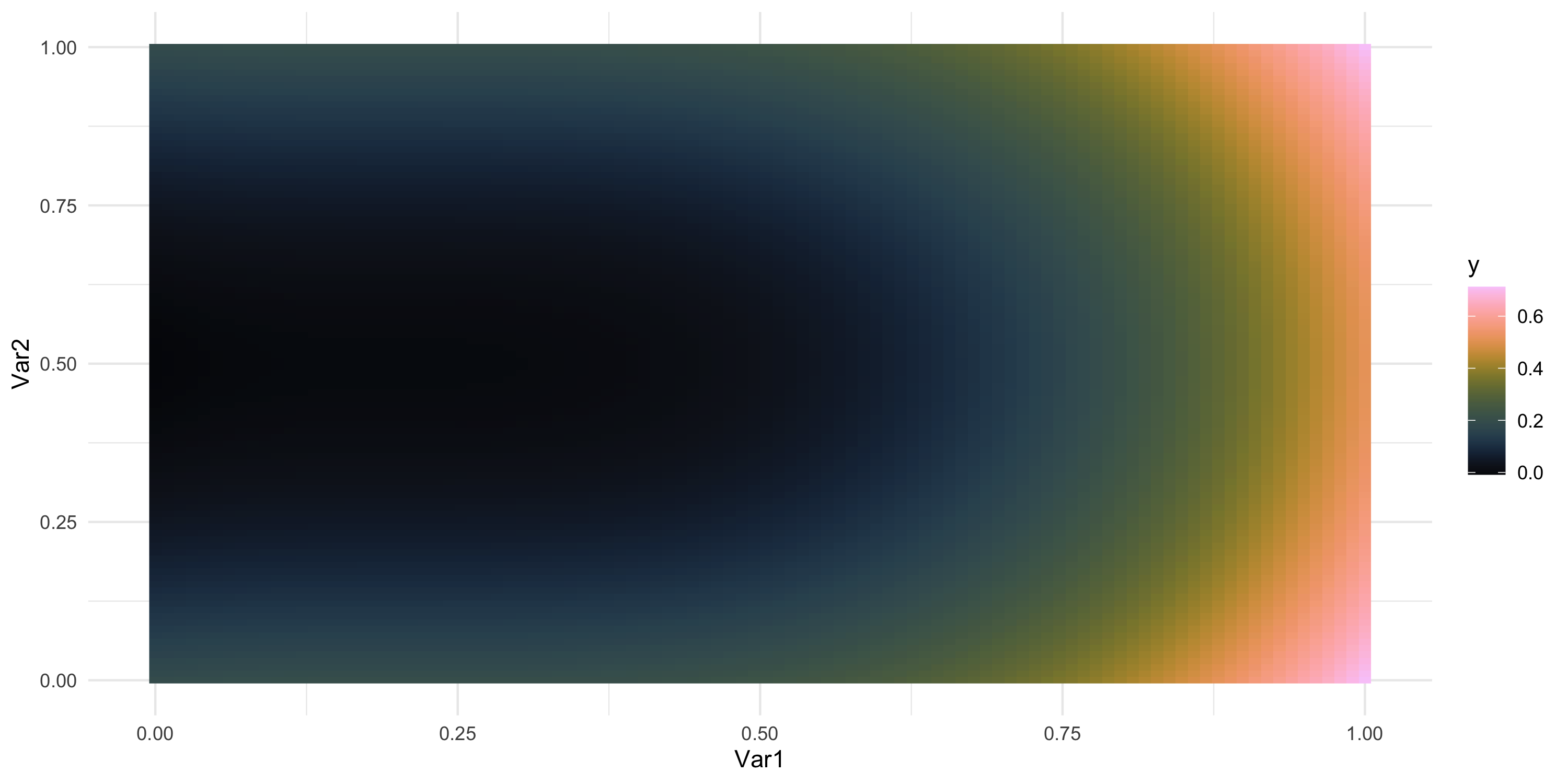
Exploratory analysis and simulation
- What does spatial dependence “look like”? Example 3
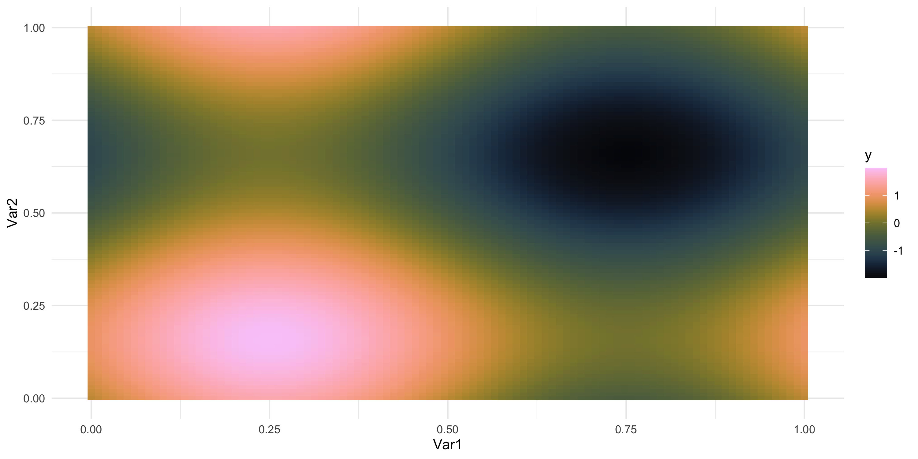
Exploratory analysis and simulation
- What does spatial dependence “look like”? Example 4
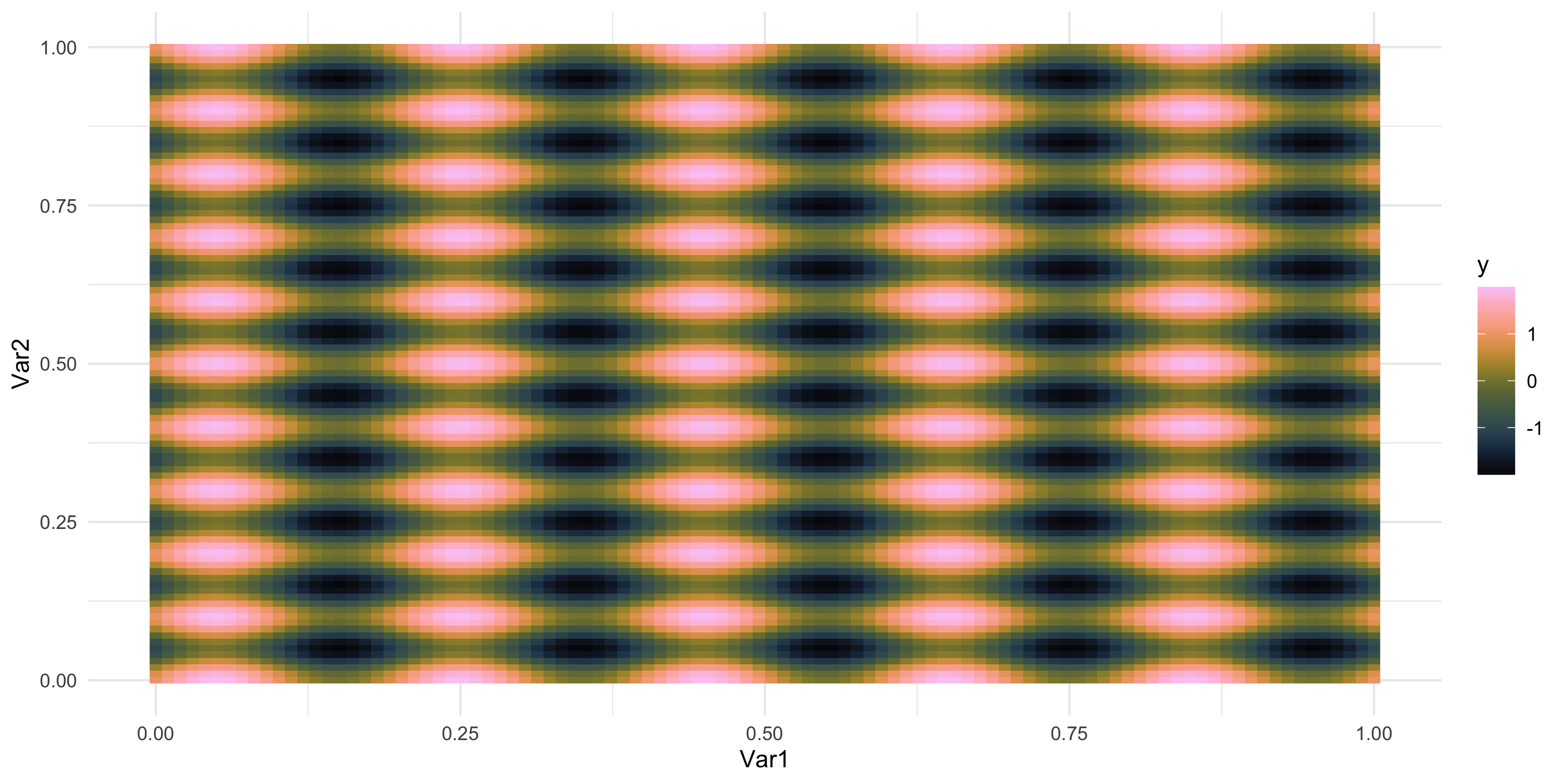
Exploratory analysis and simulation
- What does spatial dependence “look like”? Example 5
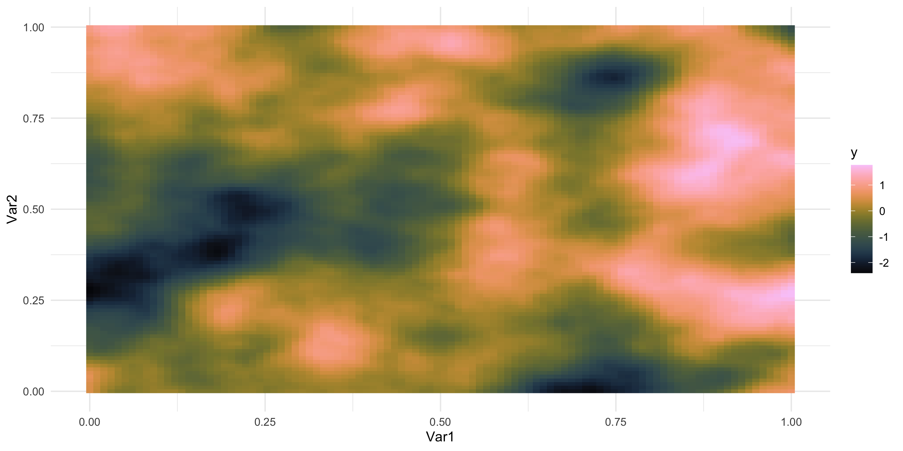
Exploratory analysis and simulation
- What does spatial dependence “look like”? Example 6
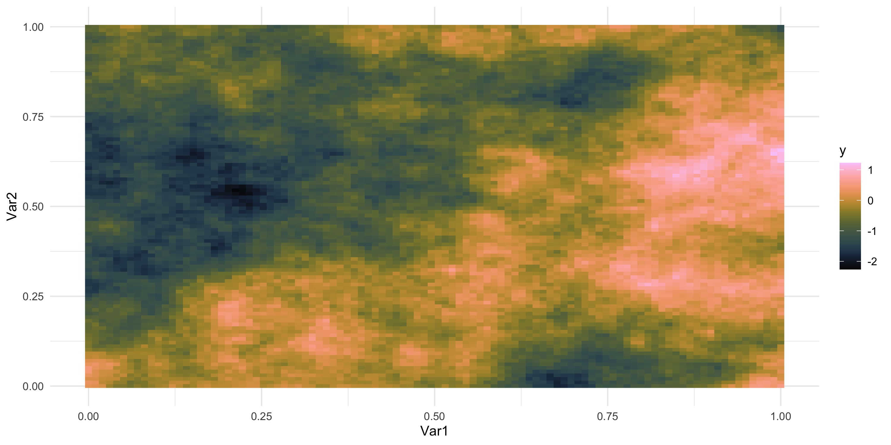
Exploratory analysis and simulation
- What does spatial dependence “look like”? Example 7
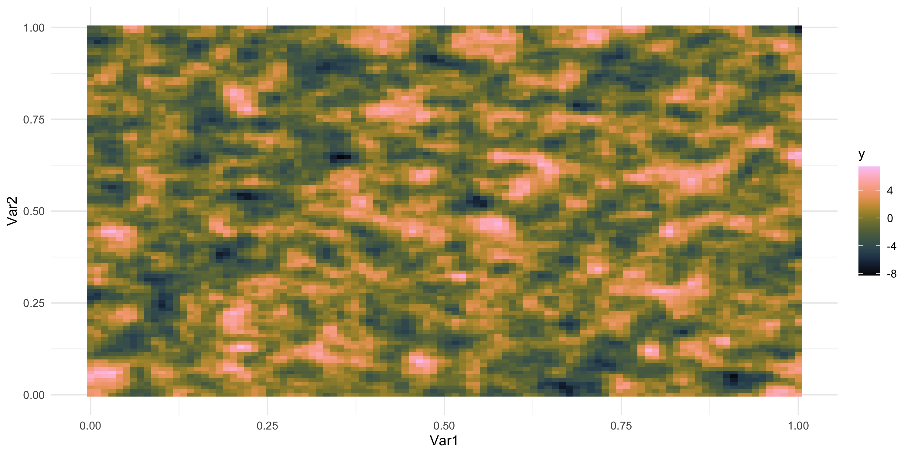
Exploratory analysis and simulation
- What does spatial dependence “look like”? Example 8
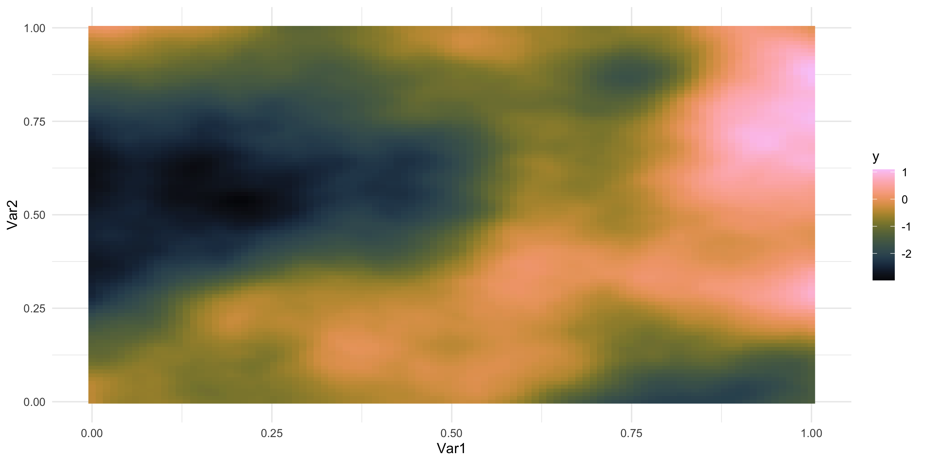
Exploratory analysis and simulation
- What does spatial dependence “look like”? Example 9
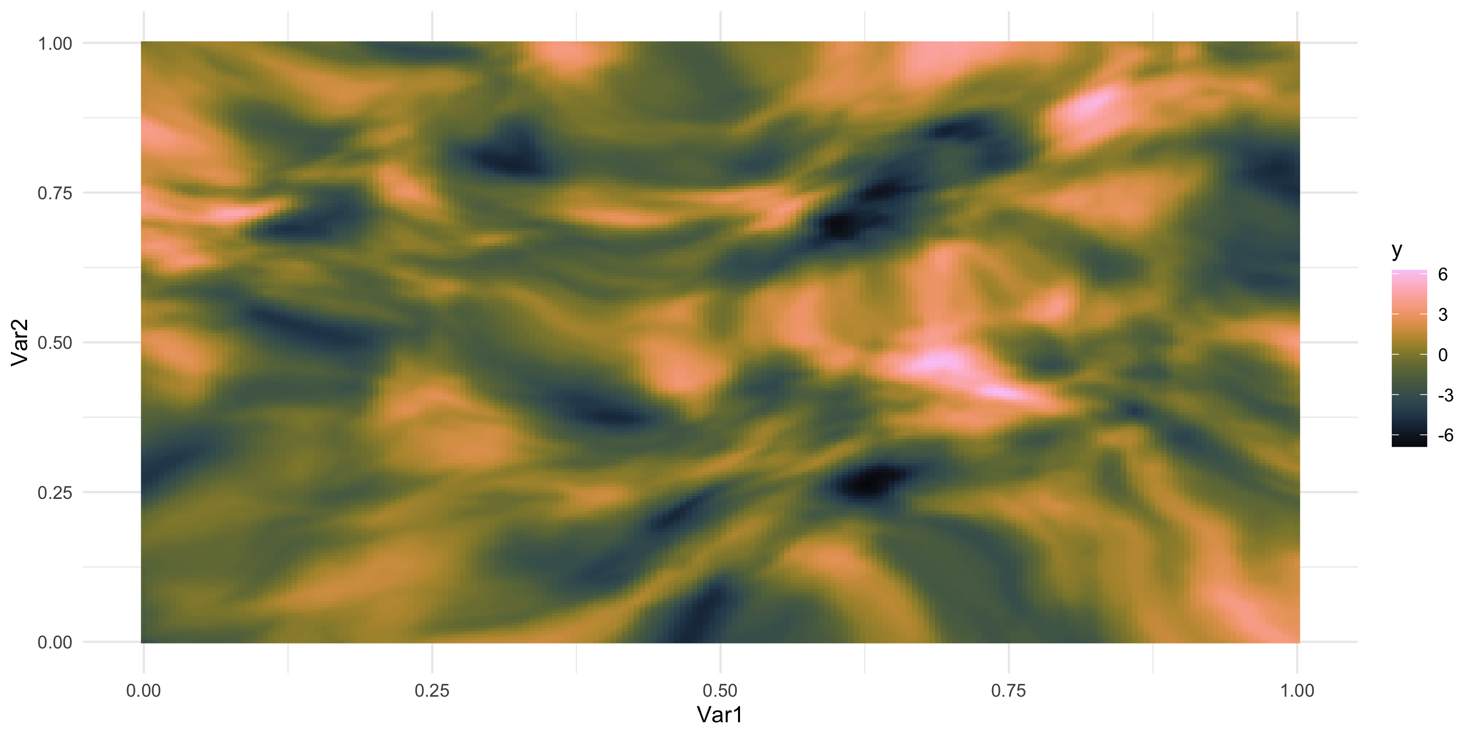
Exploratory analysis and simulation
- What does spatial dependence “look like”? Example 10
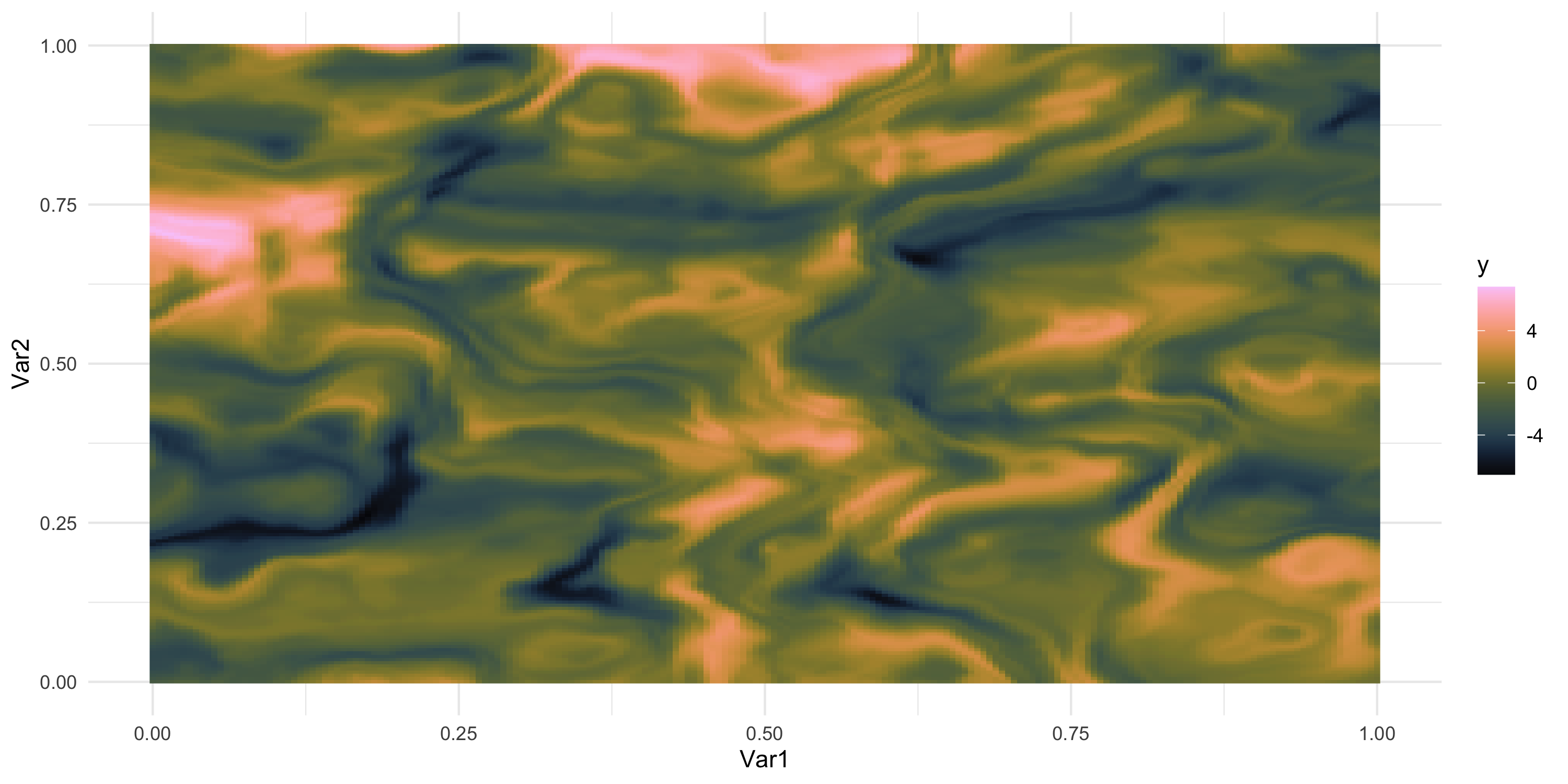
Exploratory analysis and simulation
- What common feature can we recognize?
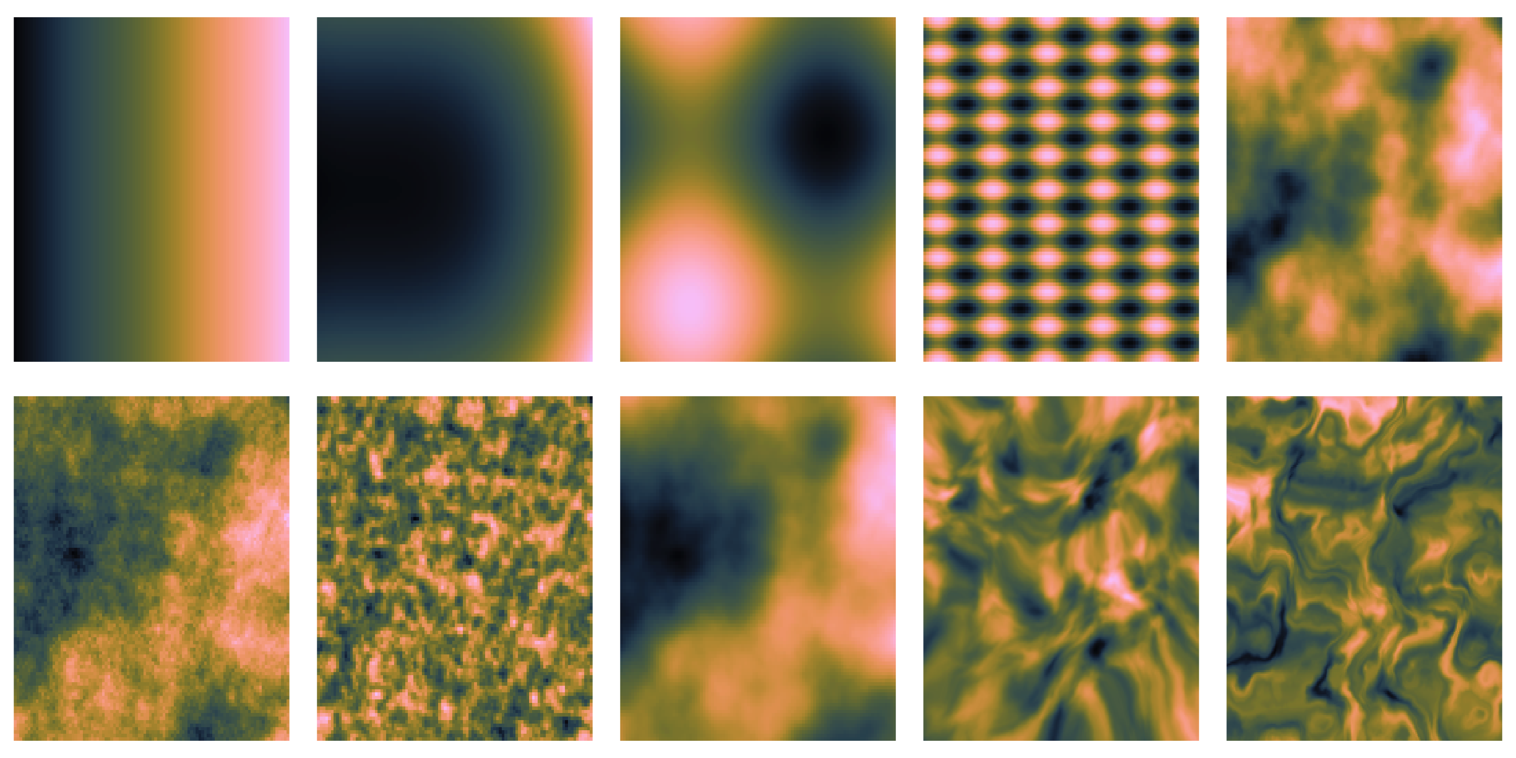
We only observe 1 sample
What if we could “re-run” the data-generation? Different data, same process
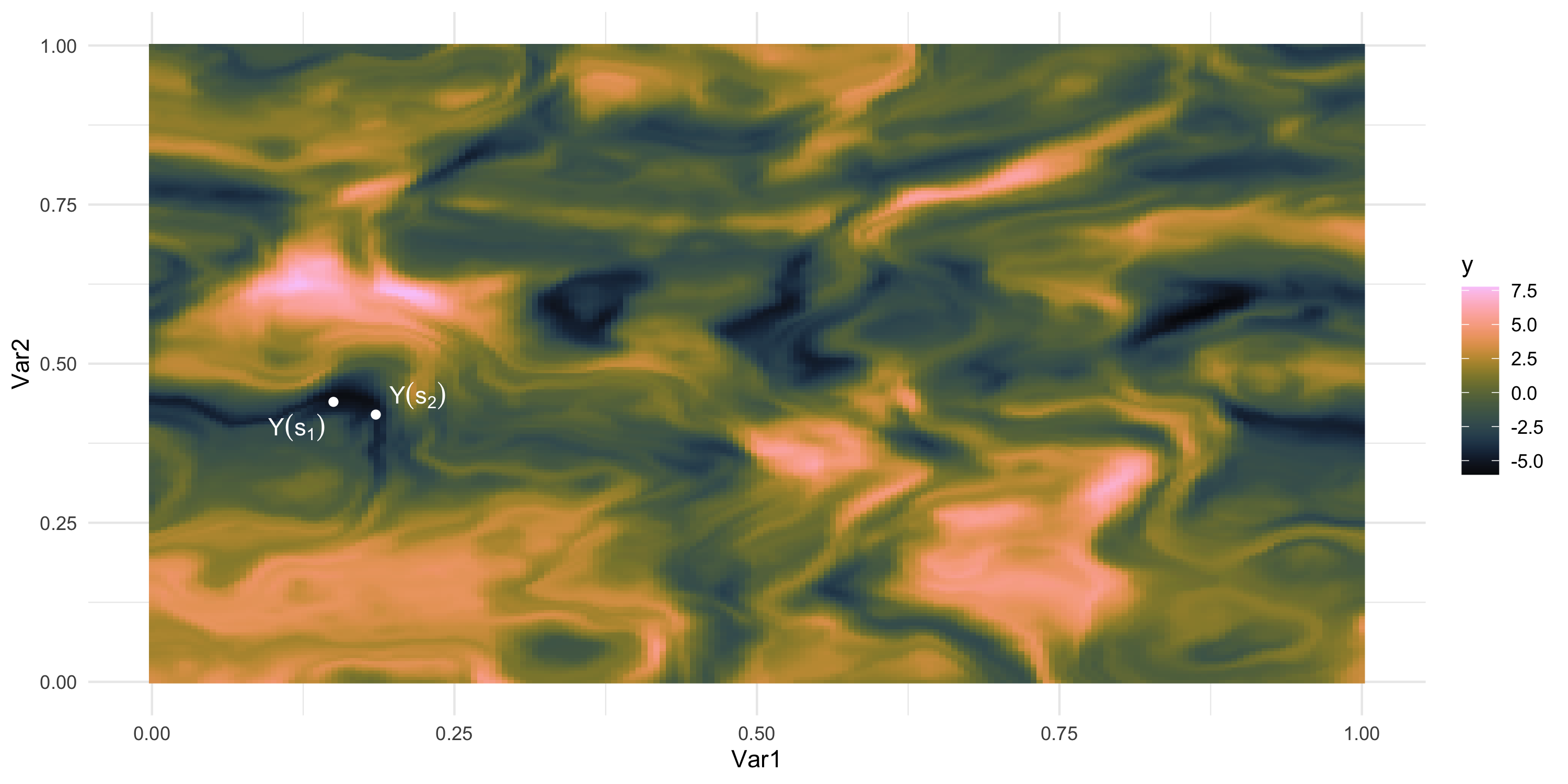
We only observe 1 sample
What if we could “re-run” the data-generation? Different data, same process
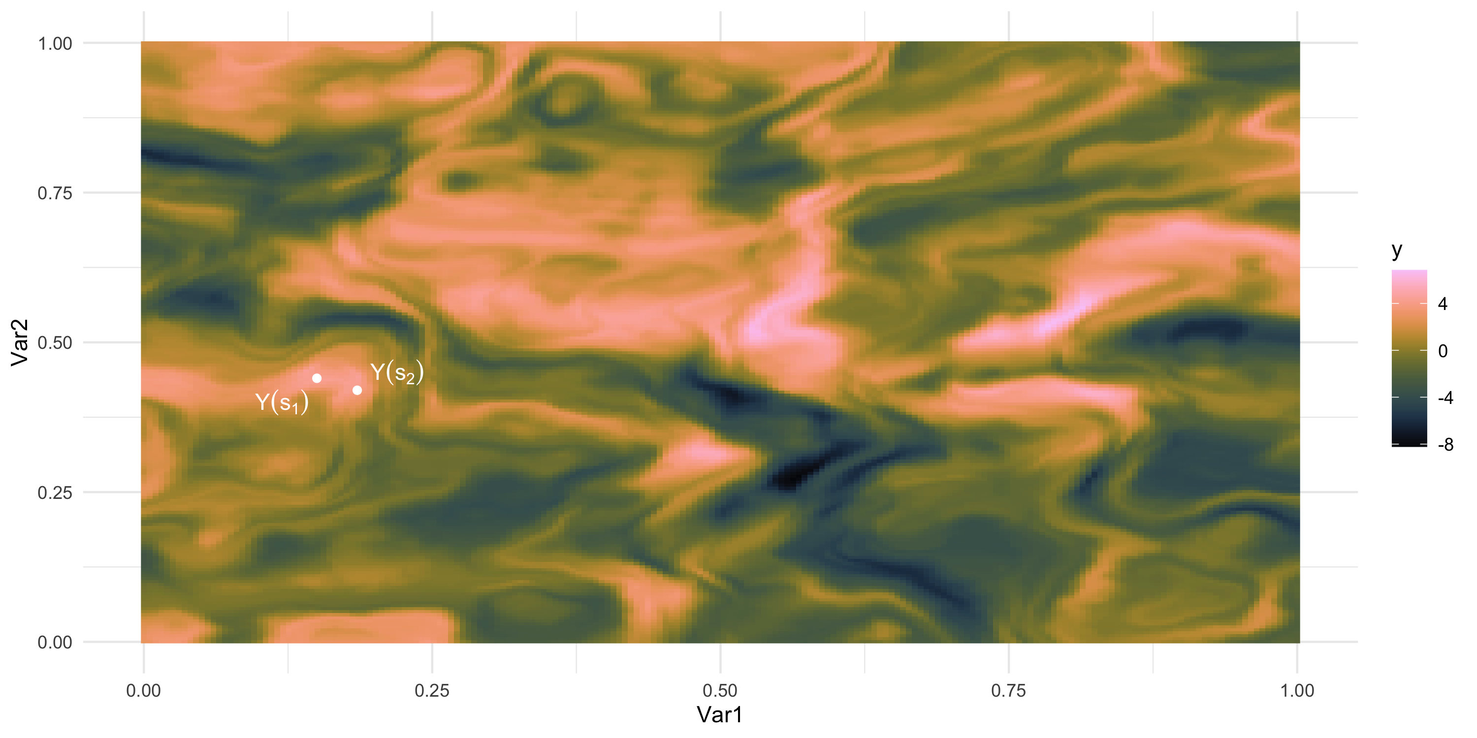
We only observe 1 sample
What if we could “re-run” the data-generation? Different data, same process
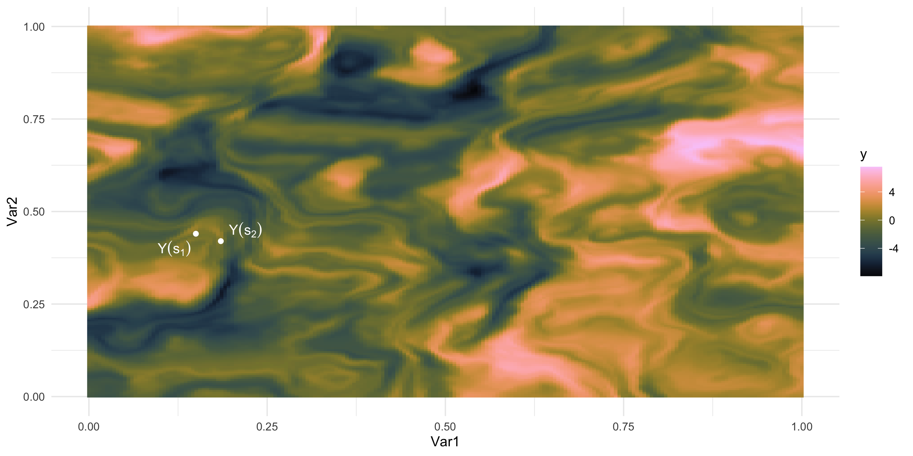
We only observe 1 sample
What if we could “re-run” the data-generation? Different data, same process
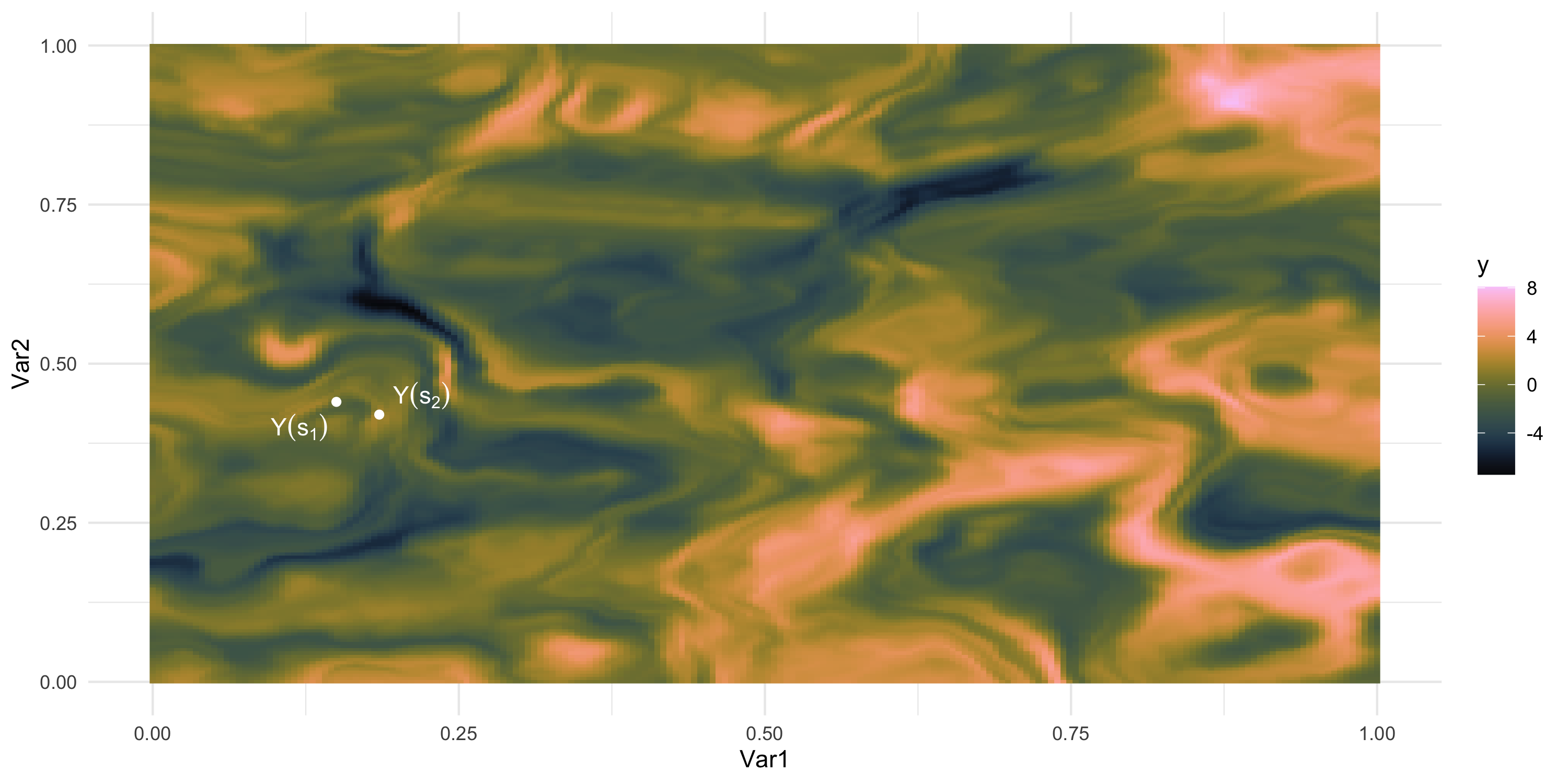
We only observe 1 sample
What if we could “re-run” the data-generation? Different data, same process
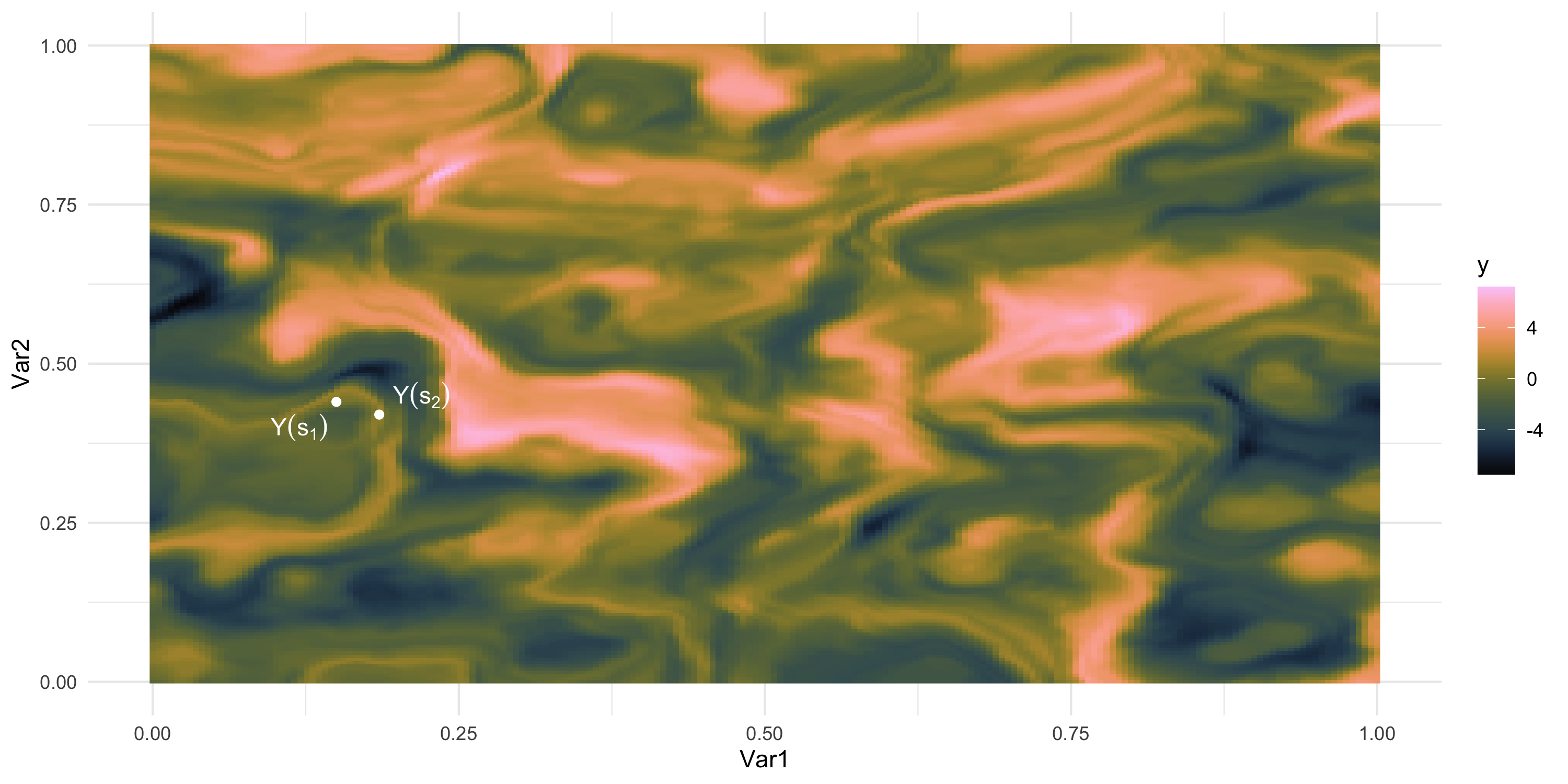
We only observe 1 sample
What if we could “re-run” the data-generation? Different data, same process
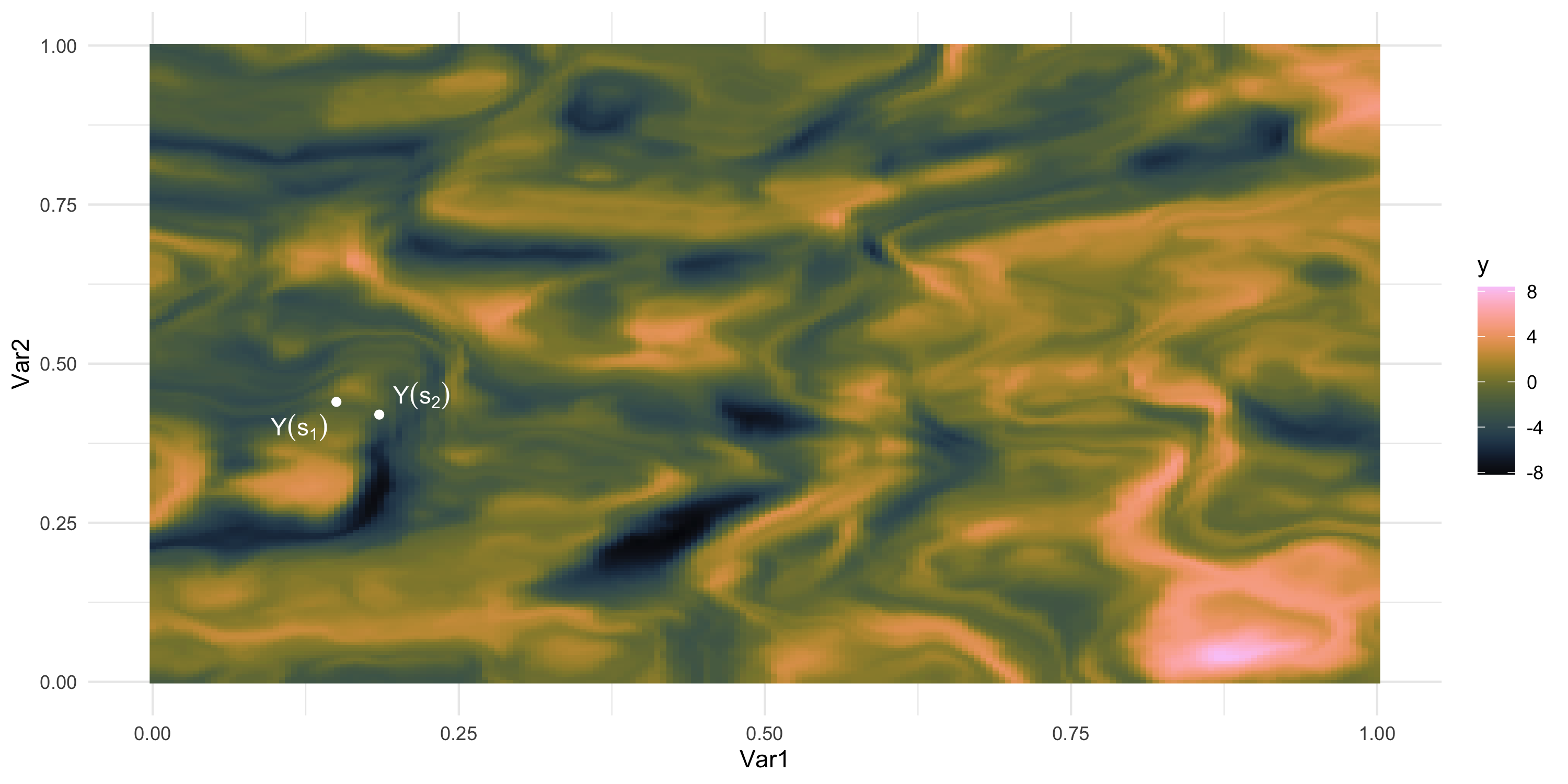
We only observe 1 sample
What if we could “re-run” the data-generation? Different data, same process
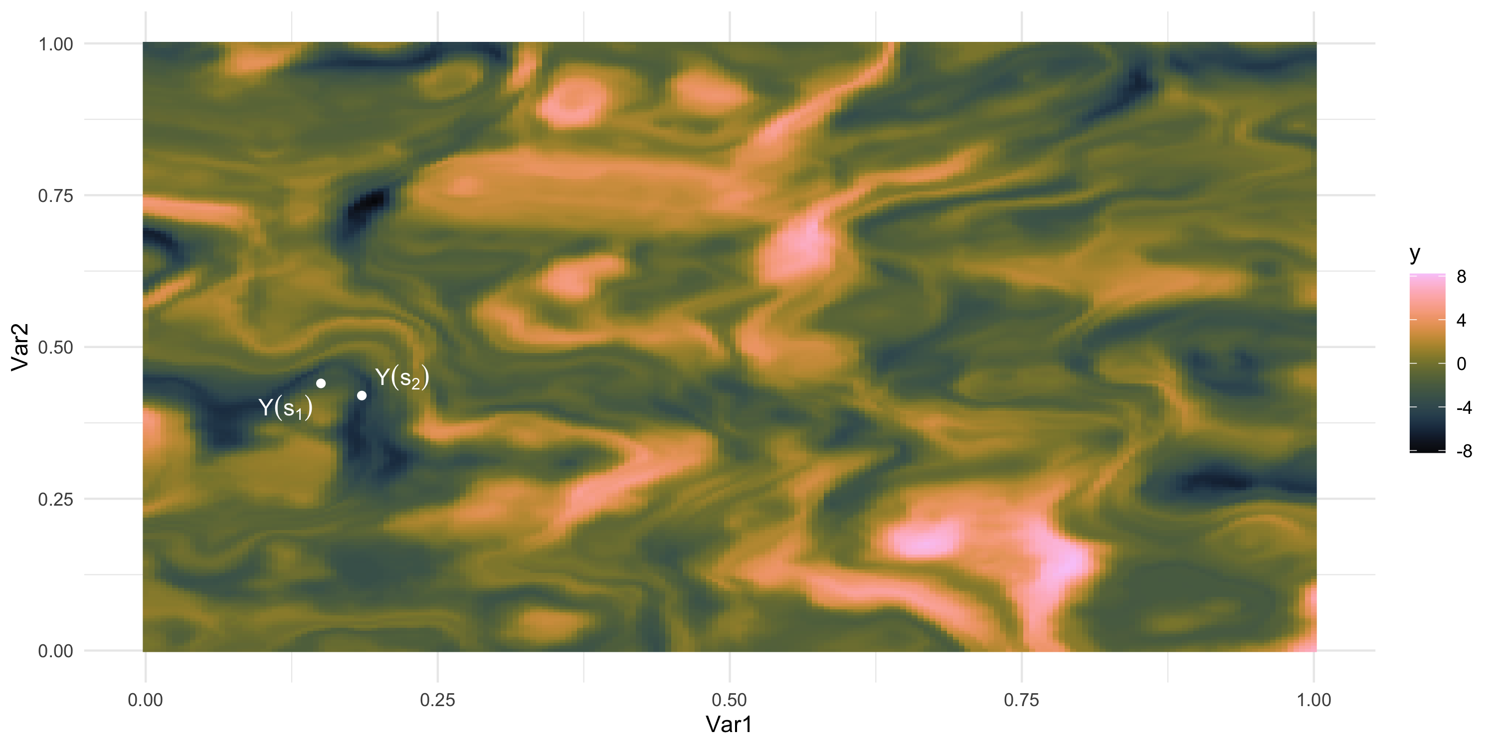
Exploratory analysis and simulation
- How “similar” are the random variables Y(s_1) and Y(s_2)?
- In other words, how large do we expect this is: | p(Y(s_2) | Y(s_1)) - p(Y(s_2)) |?
- Easier? How large do we expect this is: Cov( Y(s_1), Y(s_2) )?

Exploratory analysis and simulation
- How “similar” are the random variables Y(s_3) and Y(s_4)?
- In other words, how large do we expect this is: | p(Y(s_4) | Y(s_3)) - p(Y(s_4)) |?
- Easier? How large do we expect this is: Cov( Y(s_3), Y(s_4) )?
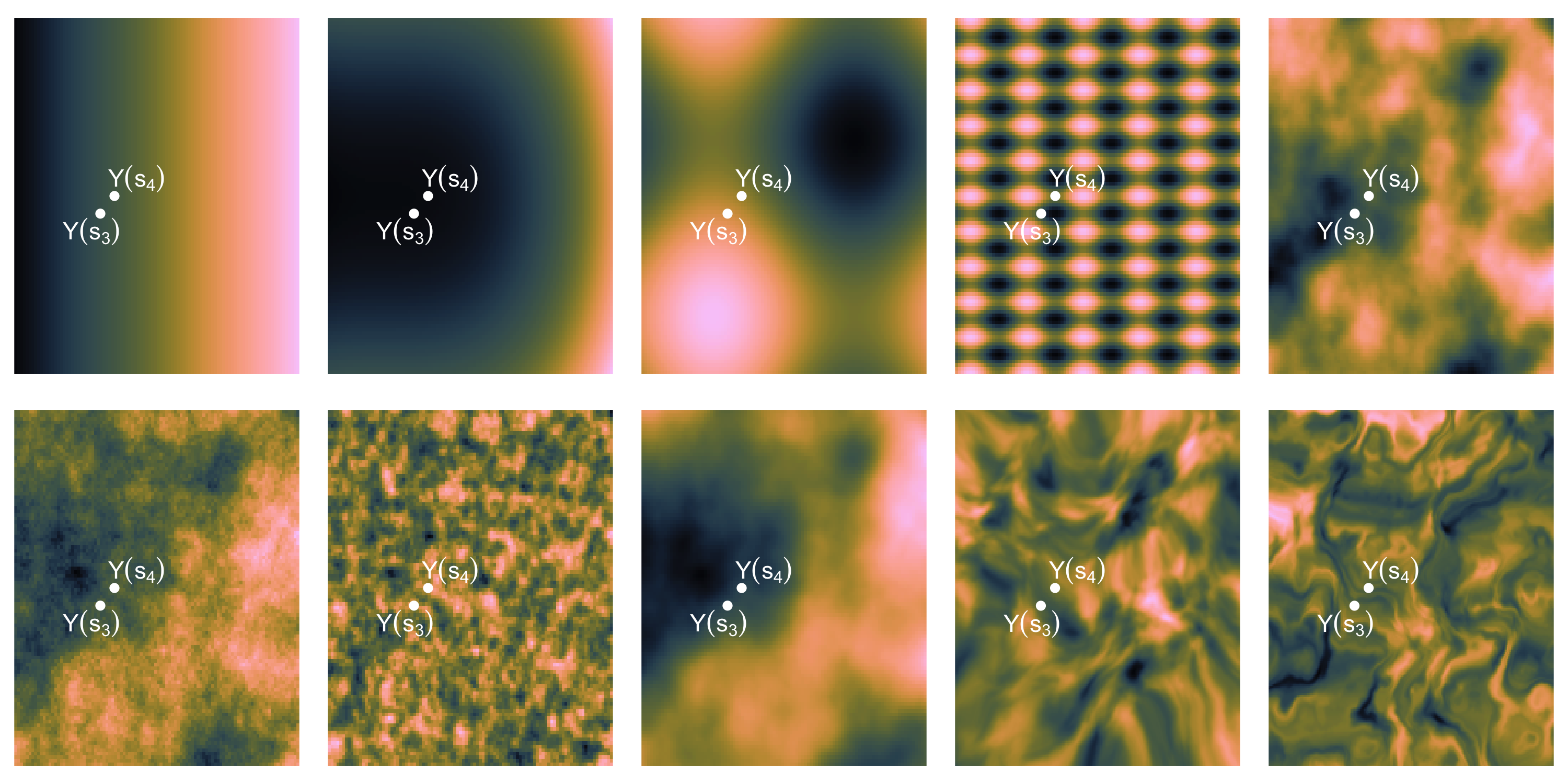
Exploratory analysis and simulation
- Distance between random variables (largely) drives how related they are
- If the variables are close to each other in space, then Cov(Y(s), Y(s')) should be larger
- The question of what model to use for Cov(Y(s), Y(s')) is crucial
- If we let Cov(Y(s), Y(s')) = g(s, s'), how do we choose g(\cdot)?
- For example, we could model g(\cdot) as a positive decreasing function of \| s-s' \|
- We can think of many other alternative models. More on this later…
Exploratory analysis: empirical semivariogram
- How do we measure spatial association in data before we attempt any sort of modeling?
- Call Y(s_i) and Y(s_j) the r.v.’s at s_i and s_j
- Suppose the domain is D = [0,1]^2
- Partition the line (0, m) \subset \Re into K disjoint intervals
- I_1 = (0=m_0, m_1], I_2 =(m_2, m_3], \dots, I_K = (m_{K-1}, m_K=m].
- Define t_k = \frac{m_k - m_{k-1}}{2} (the midpoint of the kth interval)
- Define N(t_k) = \{ (s_i, s_j) : \| s_i - s_j \| \in I_k \}
- N(t_k) is a set of all pairs of locations whose pairwise distance is “approximately” t_k
Exploratory analysis: empirical semivariogram
- Define N(t_k) = \{ (s_i, s_j) : \| s_i - s_j \| \in I_k \}
- Define the empirical semivariogram as:
\gamma(t_k) = \frac{1}{2 |N(t_k)|} \sum_{(s_i, s_k) \in I_k} (Y(s_i) - Y(s_j))^2
- What should \gamma(t) look like for increasing t if there is spatial dependence?
- If spatial dependence, Y(s_i) and Y(s_j) should be close to each other if s_i and s_j are not far apart
- We then expect \gamma(t) to be increasing with t: as the locations are farther from each other, the observations become increasingly different
Exploratory analysis: empirical semivariogram
install.packages("geoR")(you may need to install XQuartz in your system)- Plot the empirical semivariogram via
geoR::variog - Let’s use Example 8 from earlier
sv <- simdf %>% with(geoR::variog(data = y, coords = cbind(Var1, Var2), messages=FALSE))

sv_df <- data.frame(dists = sv$u, variogram = sv$v, npairs = sv$n, sd = sv$sd)
sv_plot <- ggplot(sv_df, aes(x=dists, y=variogram)) + geom_point(size=2, shape=8) +
  theme_minimal()

grid.arrange(data_plot, sv_plot, nrow=1)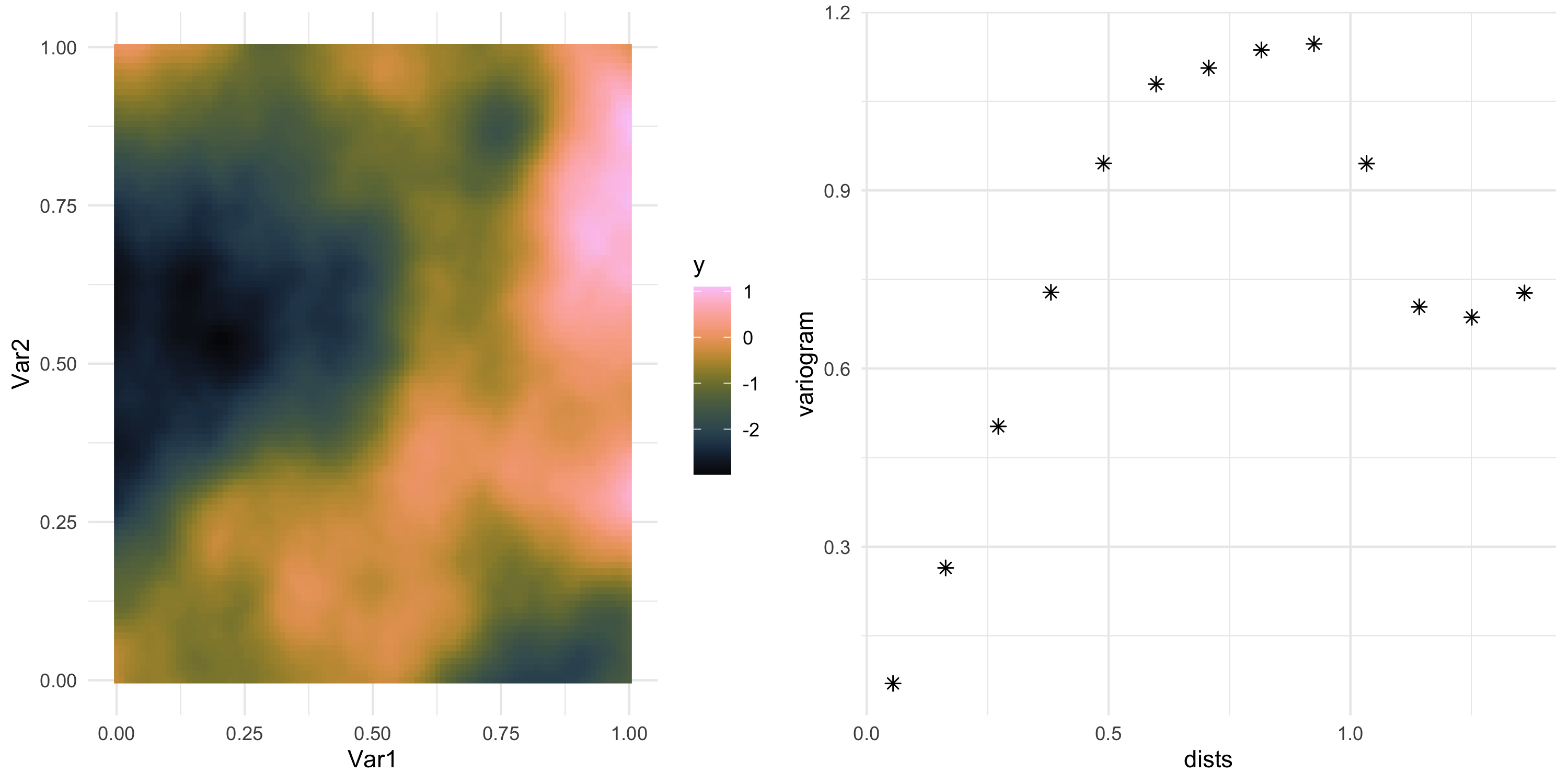
Exploratory analysis: empirical semivariogram
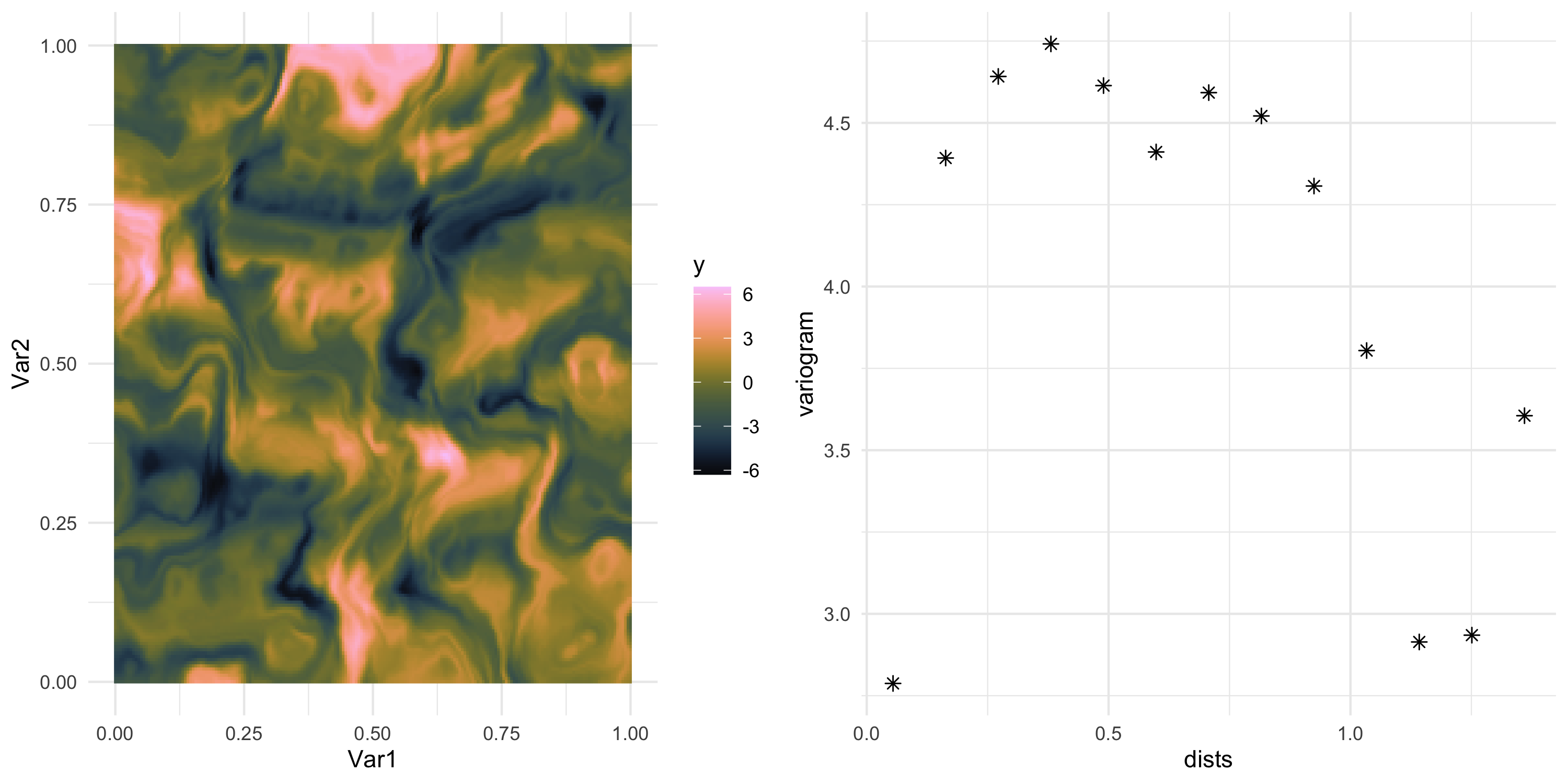
- Let’s use Example 10 from earlier
Exploratory analysis: example
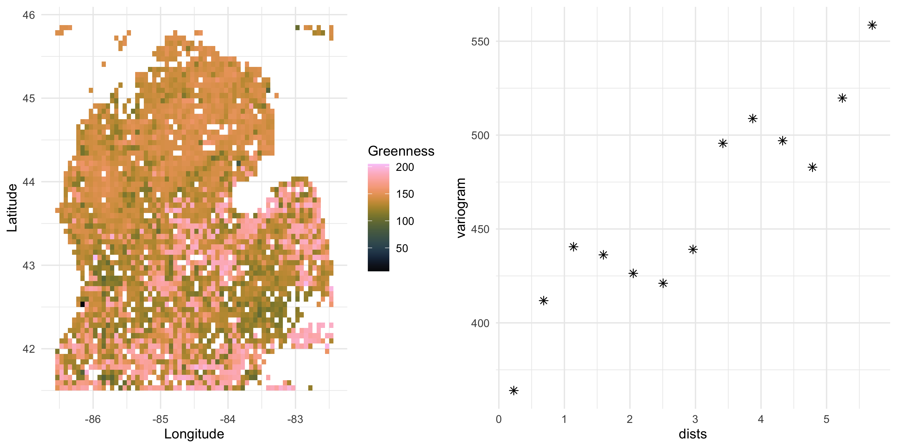
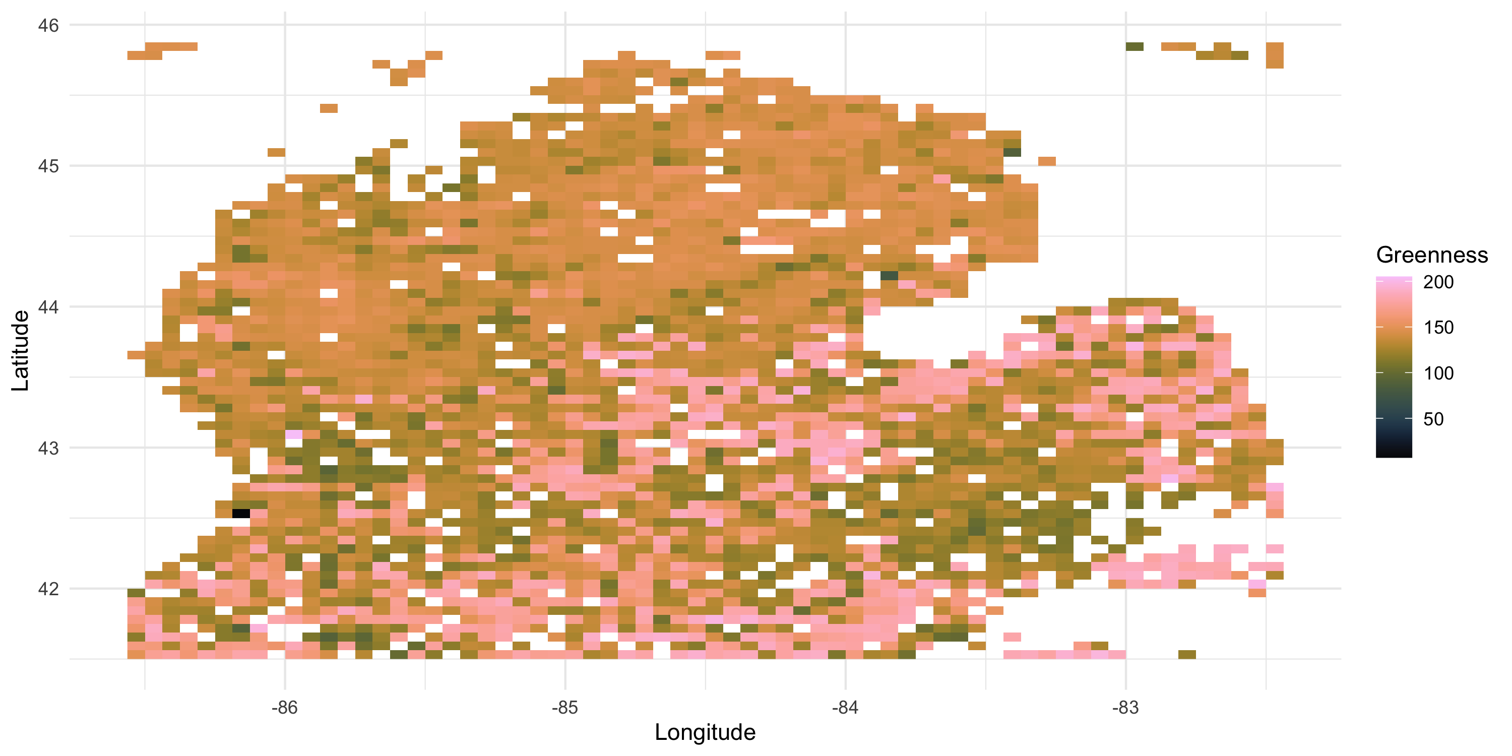
- We want to investigate a variable representing the time it takes for vegetation to reach peak greenness
- Changes in the greenup time may be explained by climate change
Exploratory analysis: example
sv <- df %>% with(geoR::variog(data = Greenness, coords = cbind(Longitude, Latitude), messages=FALSE))
sv_df <- data.frame(dists = sv$u, variogram = sv$v, npairs = sv$n, sd = sv$sd)
sv_plot <- ggplot(sv_df, aes(x=dists, y=variogram)) + geom_point(size=2, shape=8) +
  theme_minimal()

grid.arrange(data_plot, sv_plot, nrow=1)