Group challenge 1: Example
Spatial Statistics - BIOSTAT 696/896
Michele Peruzzi
University of Michigan
Introduction
- We consider a scientific problem in the area of whateverology
- Data on this topic are available at website https://whateverology.idk
- Specifically we target the study of ABC, using data https://whateverology.idk/ABC.csv
- The dataset is a point-referenced dataset of 5000 observations
Data overview
- The dataset is of dimension 5000, 5; in addition to latitude and longitude, it includes variables
x, y, and z
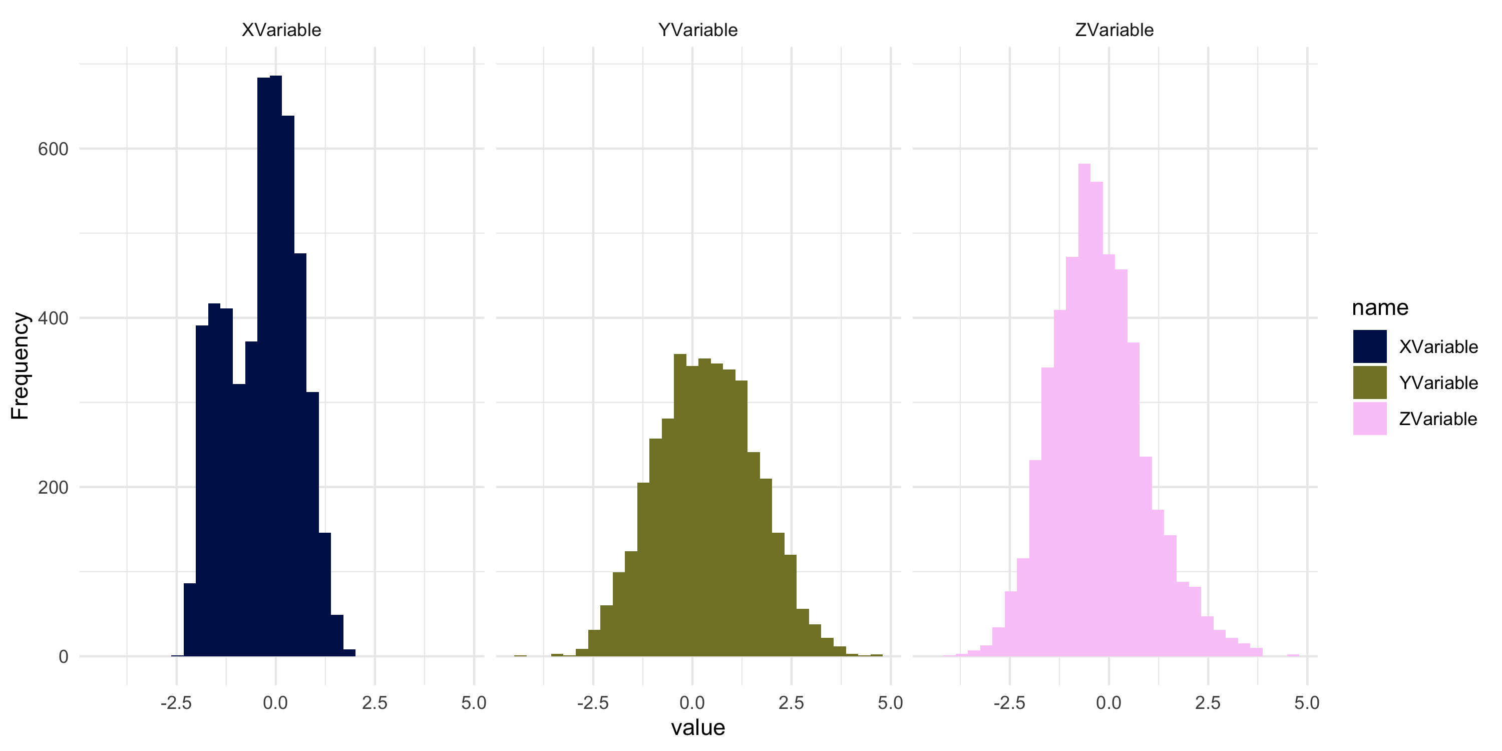
- A histogram of all variables they are all roughly centered at zero
![]()
Data overview
- Variable Y is missing at 20.3 percent of total locations
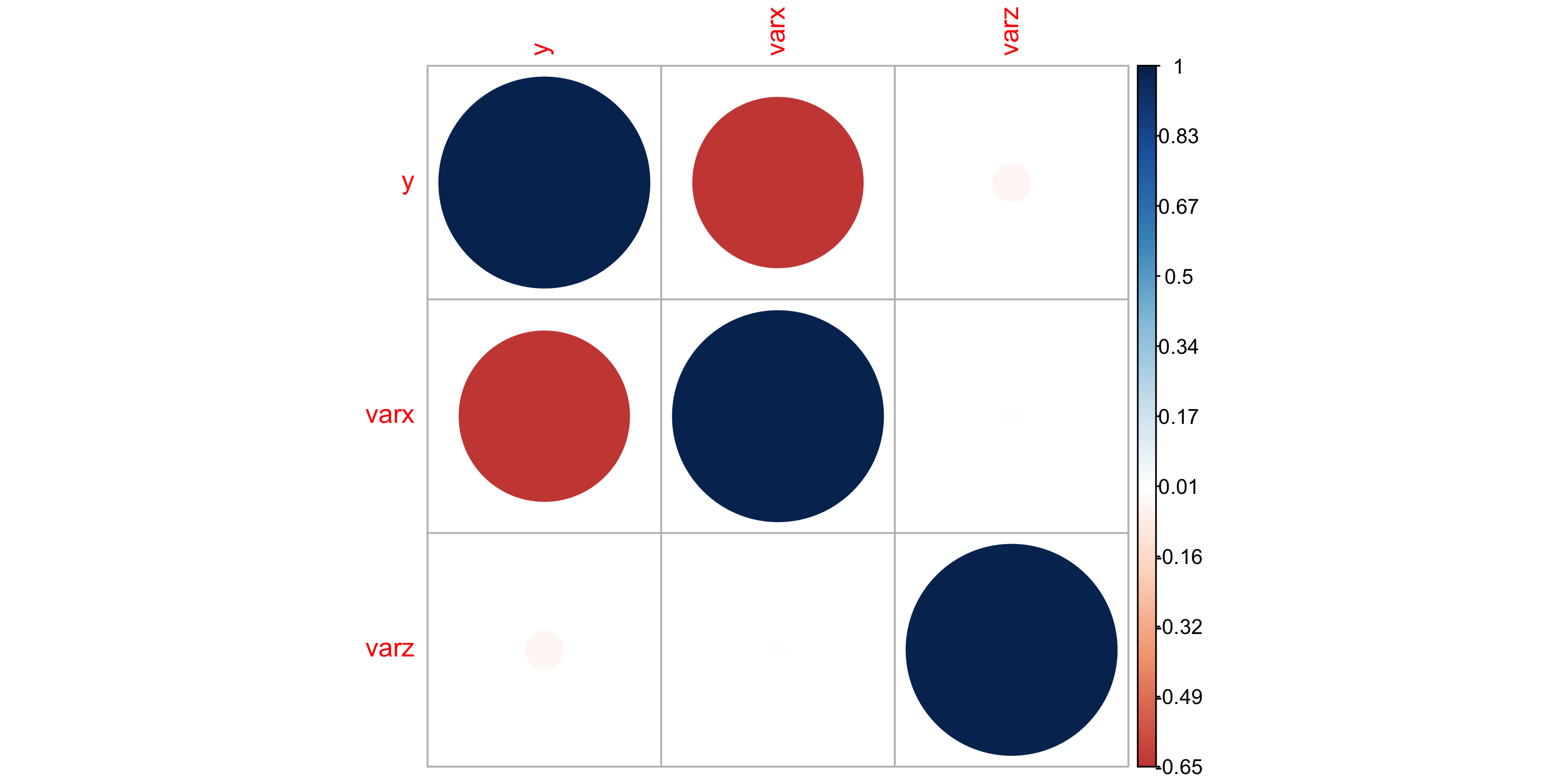
- Variables X and Y are linearly negatively correlated
- Variable Z seems unrelated to the other two
![]()
Data type and locations
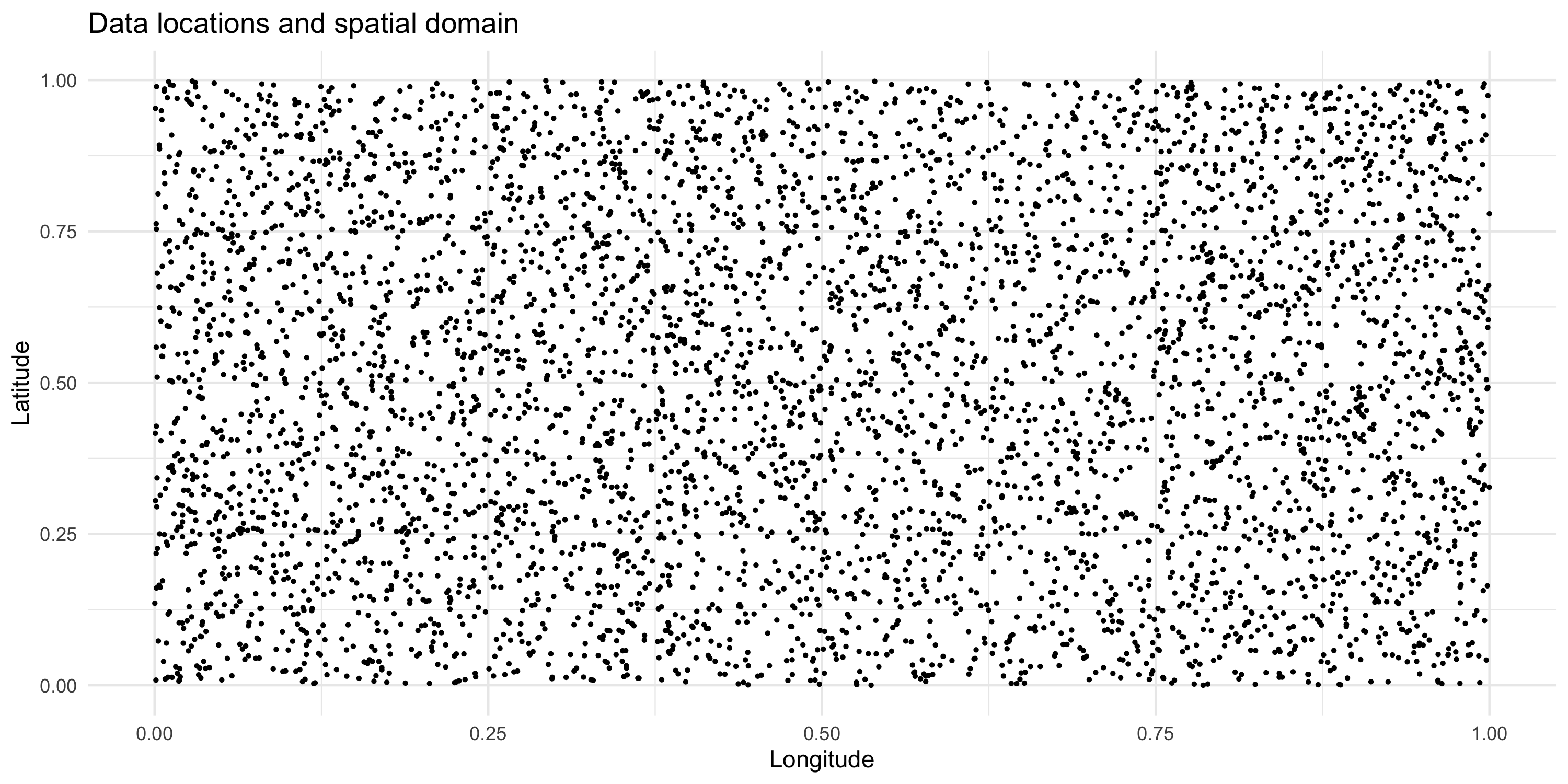
- Data locations cover the spatial domain with uniformity
- We consider the variables X and Y over the domain D
![]()
More visualization
- We visualize interesting features of the data!
[Here]
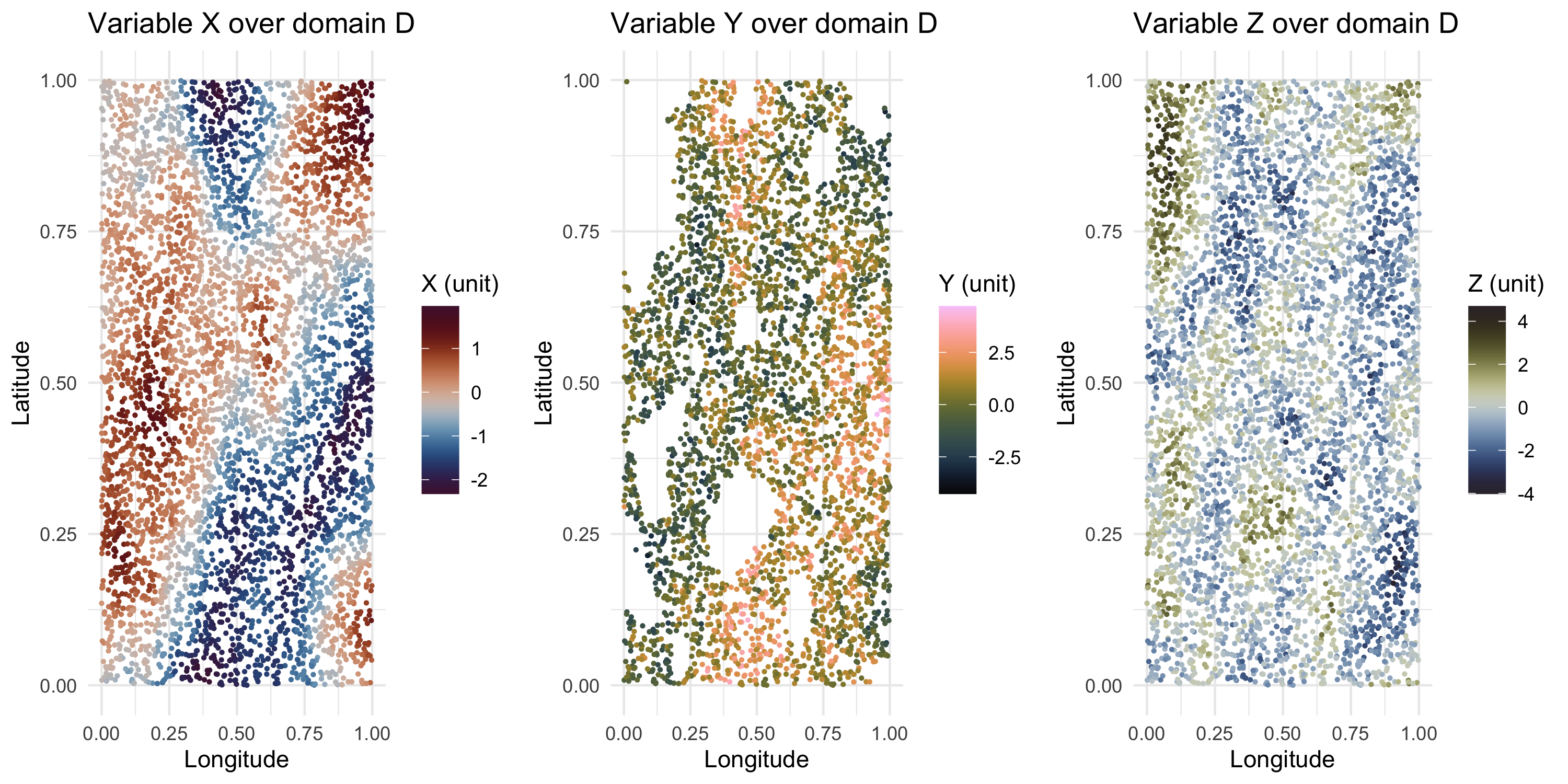
Maps of the data
![]()
Explaining Y via X
- By inspecting the maps of X and Y we see that there may be a negative association between them
- This makes sense because X explains Y in a certain way according to scientific knowledge
- However, we note that Y is missing in some large areas where X is available
- Further investigation to figure out whether missingness may impact results
- Value of Z may relate to whether Y is missing. We explain this with…
Brainstorming models for this dataset
- We think X \to Y and Z \to Y
- We consider X and Z as covariates
- The measurements of Y are reasonably noisy
- Y has spatial variability that may not be fully explained by X and Z
- Therefore, the DAG could look like \theta \to Y, \tau \to Y where the former is a vector of unknown parameters describing spatial dependence, \tau is an unknown scalar which refers to how precise our measurements of Y are in this dataset
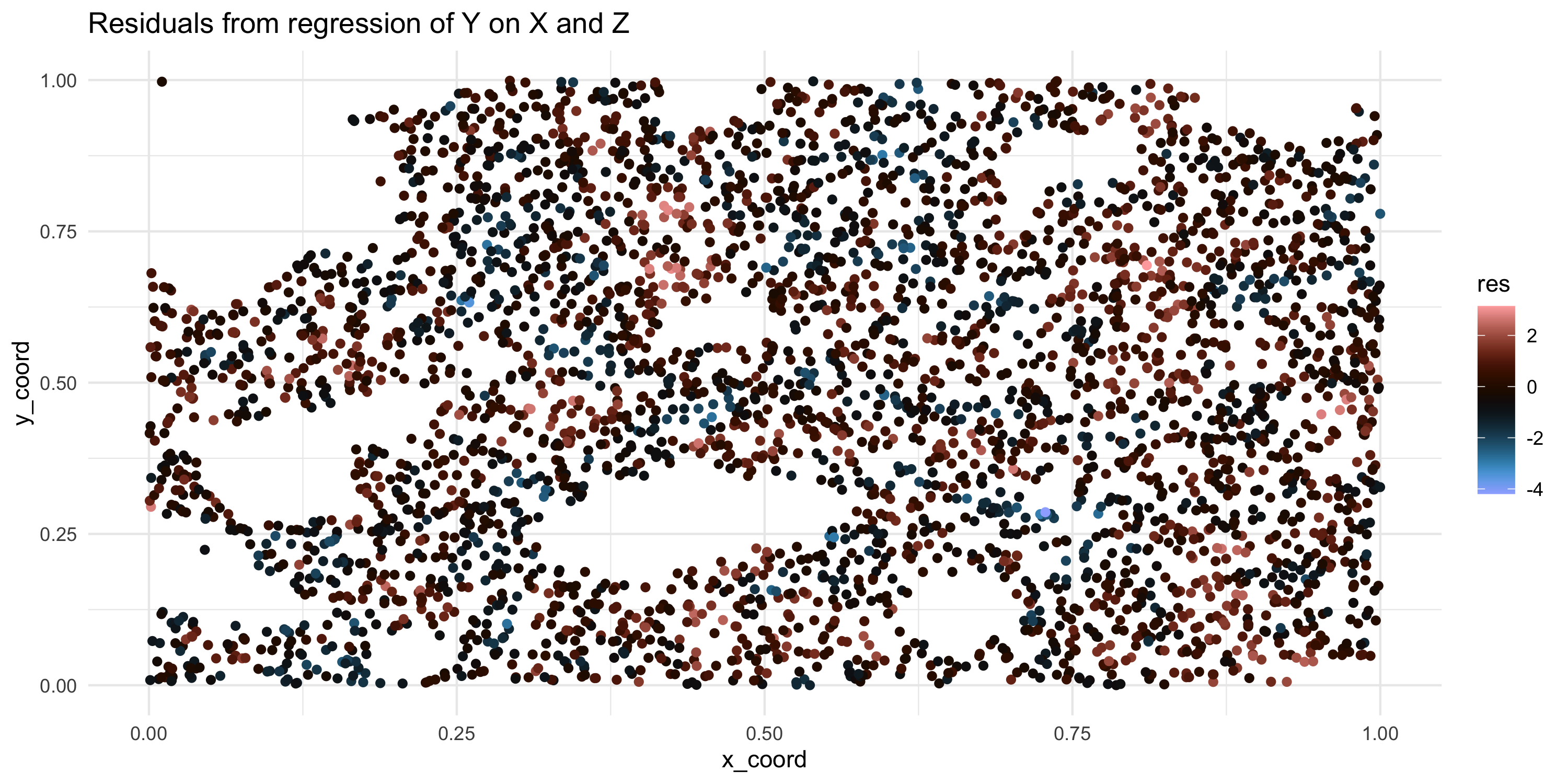
Preliminary analysis
- We consider a linear regression of X and Z on Y
- Coefficients on X and Z are -0.943137 and -0.0409616, respectively
- P-value for coefficient on X is very small, and the one on Z is statistically significantly different from zero at 5% confidence
- However, we are unsatisfied with this analysis because the residuals show significant spatial variability
- Because X and Z alone do not satisfactorily explain all variability in Y, we need to conduct more analyses
![]()
Concluding words
- We have identified a potential route for modeling this dataset by explaining variability of Y via X and Z
- Preliminary analyses seem to confirm this relationship
- Simple linear regression is unable to capture all spatial variability
- We target the development of a more complex model incorporating spatial variability
- The fact that spatial variability remains important makes sense: Y can be explained by variable W, which is not in this dataset
- The unobserved variable W has an intuitive spatial pattern that may resemble the spatial pattern of regression residuals
- Our proposed intuitive model ignores the fact that missingness of Y may be explained by Z but we believe our assumption is reasonable because…